【雷达通信】滤波及数据融合【滤波包括了常增益滤波、卡尔曼（Kalman）滤波和扩展卡尔曼滤波（EKF） 数据融合采用BC和CC两种，基于KF和EKF实现】（Matlab代码实现）

 👨‍🎓个人主页：研学社的博客 

💥💥💞💞欢迎来到本博客❤️❤️💥💥

🏆博主优势：🌞🌞🌞博客内容尽量做到思维缜密，逻辑清晰，为了方便读者。

⛳️座右铭：行百里者，半于九十。

📋📋📋本文目录如下：🎁🎁🎁

目录

💥1 概述

📚2 运行结果

2.1 EKF

        2.2 过滤器2D 

🎉3 参考文献

🌈4 Matlab代码实现

---

💥1 概述

随着5G时代的到来,商业通信服务呈现爆炸式增长,导致本就有限的频谱资源变得更加拥塞与稀缺。为最大限度地利用稀缺频谱,出现了允许单个系统同时适应雷达和通信功能的技术。

本文实现滤波及数据融合【滤波包括了常增益滤波、卡尔曼（Kalman）滤波和扩展卡尔曼滤波（EKF） 数据融合采用BC和CC两种，基于KF和EKF实现】

📚2 运行结果

2.1 EKF

 

 

 

 

 

 

 

 

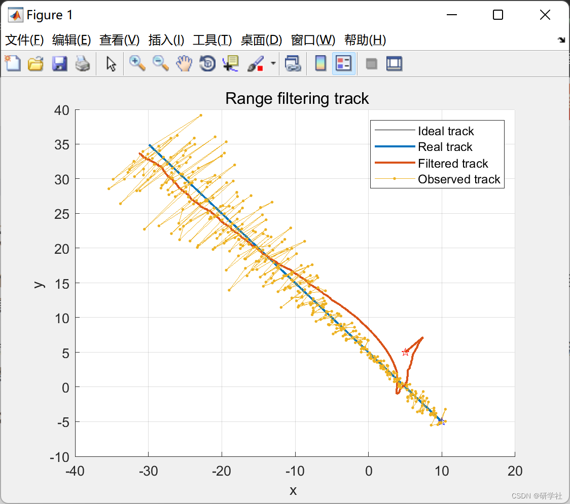
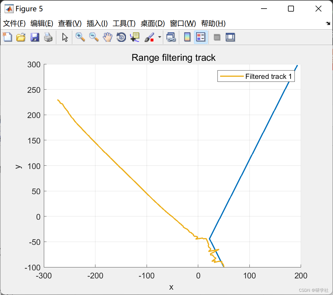
2.2 过滤器2D 

 

 

 

 

 

 

 

 部分代码：

sigma = 1;
noise = randn(2,N).*sigma;
%initial data
X = zeros(4,N);
Z = zeros(2,N);
X(:,1) = [0, 5, 0, 10];
Z(:,1) = [X(1,1),X(3,1)];
sigma_error=[1,1];

a = 0.3;                %alpha 0.3-0.5
b = 2*(2-a)-4*sqrt(1-a);%beta, determined by alpha
K = [a, b/T, 0, 0
     0, 0, a, b/T]';           %filter gain
%transition matrix
F = [1 T 0 0 
     0 1 0 0
     0 0 1 T
     0 0 0 1];
%observation matrix
H = [1 0 0 0 
     0 0 1 0];

%real & observed data
for n=2:N
    X(:,n) = F * X(:,n-1);
    Z(:,n) = H * X(:,n) + noise(:,n);
end
figure;
hold on;grid on;
plot(X(1,:),X(3,:),'LineWidth',2);
plot(Z(1,:),Z(2,:),'.-');

X_update = zeros(4,N);
X_update(:,1) = X(:,1); 
%filter
a = [0 0.1 0.3 0.5 1];  

for n=2:N
    X_p = F * X_update(:,n-1);
    Z_p = H * X_p;
    X_update(:,n) = X_p + K*(Z(:,n)-Z_p);
end

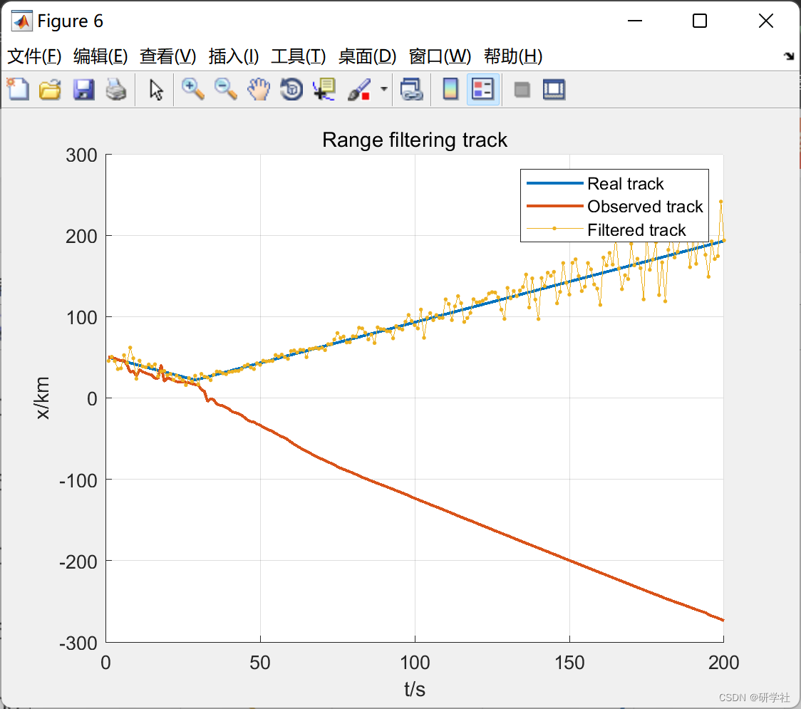
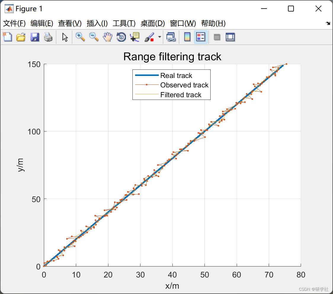
plot(X_update(1,:),X_update(3,:));
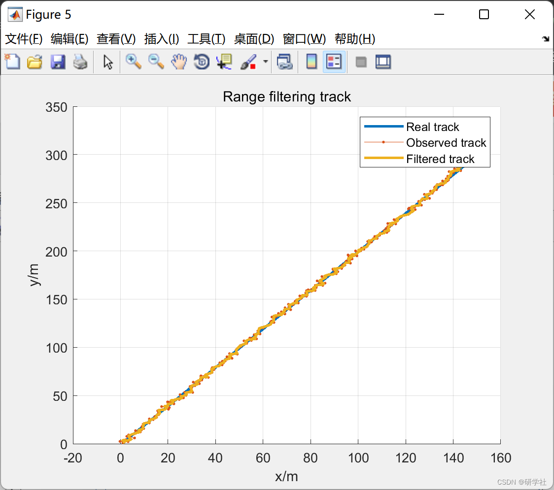
xlabel('x/m');ylabel('y/m');legend('Real track','Observed track','Filtered track');
title('\fontsize{14}Range filtering track')

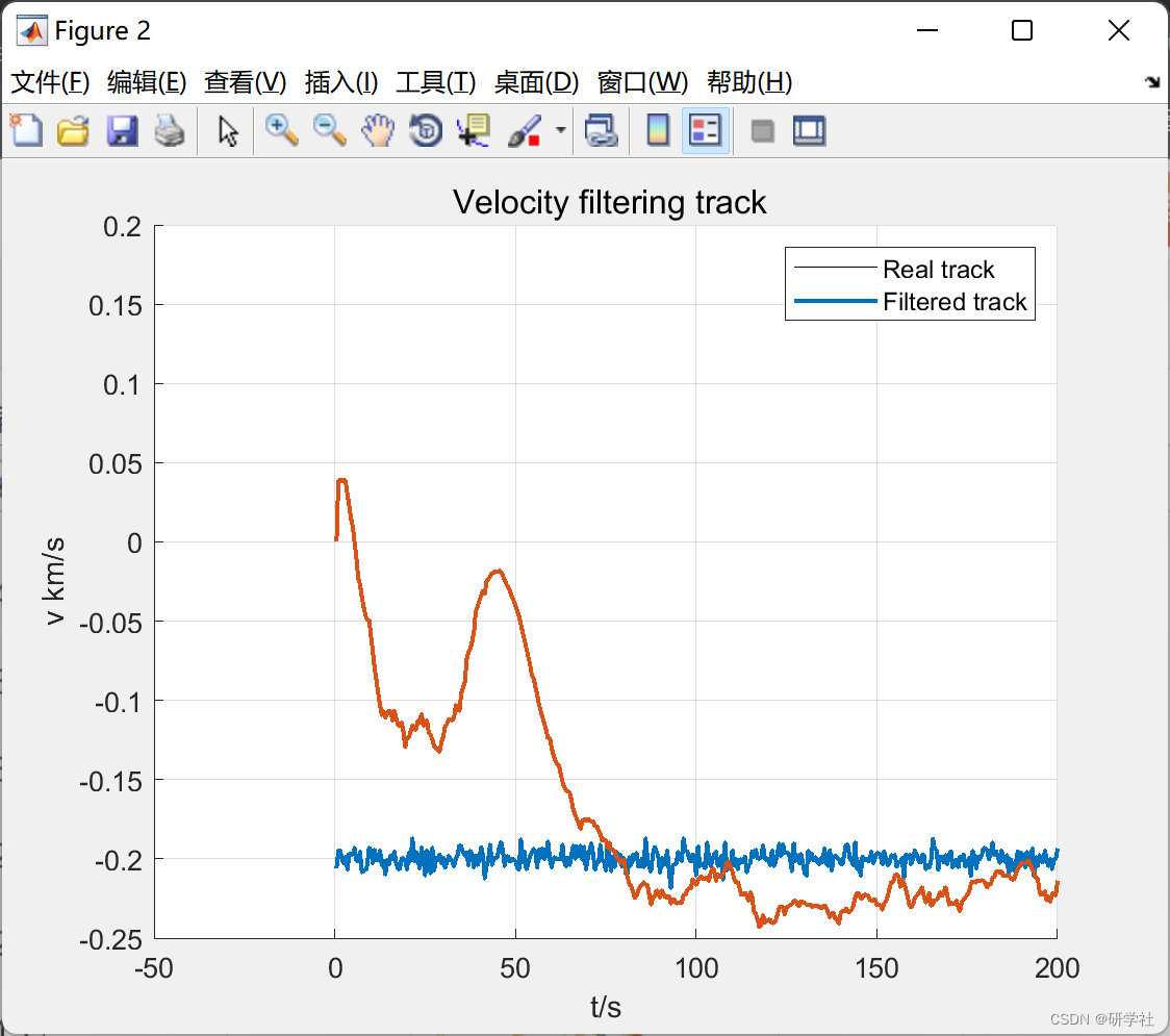
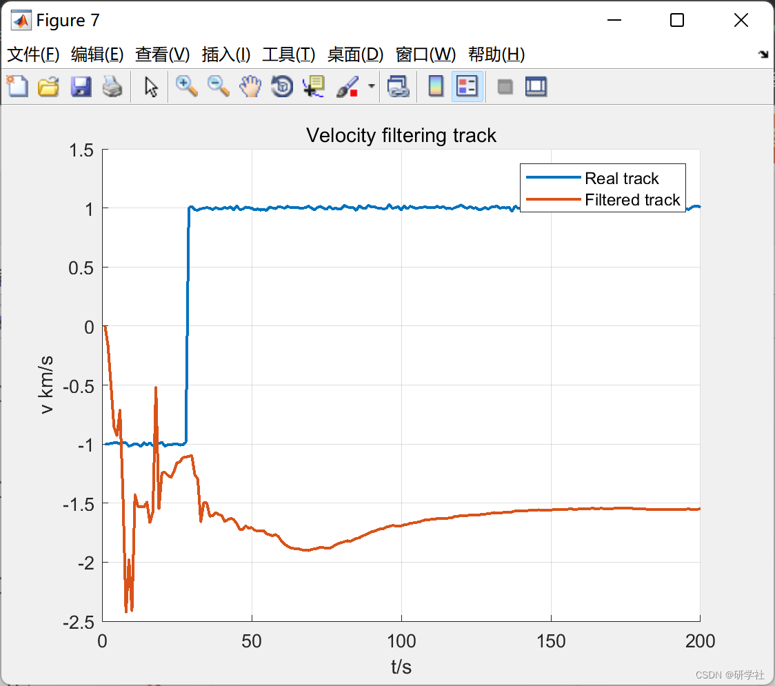
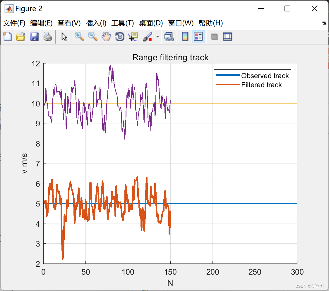
figure;
hold on;grid on;
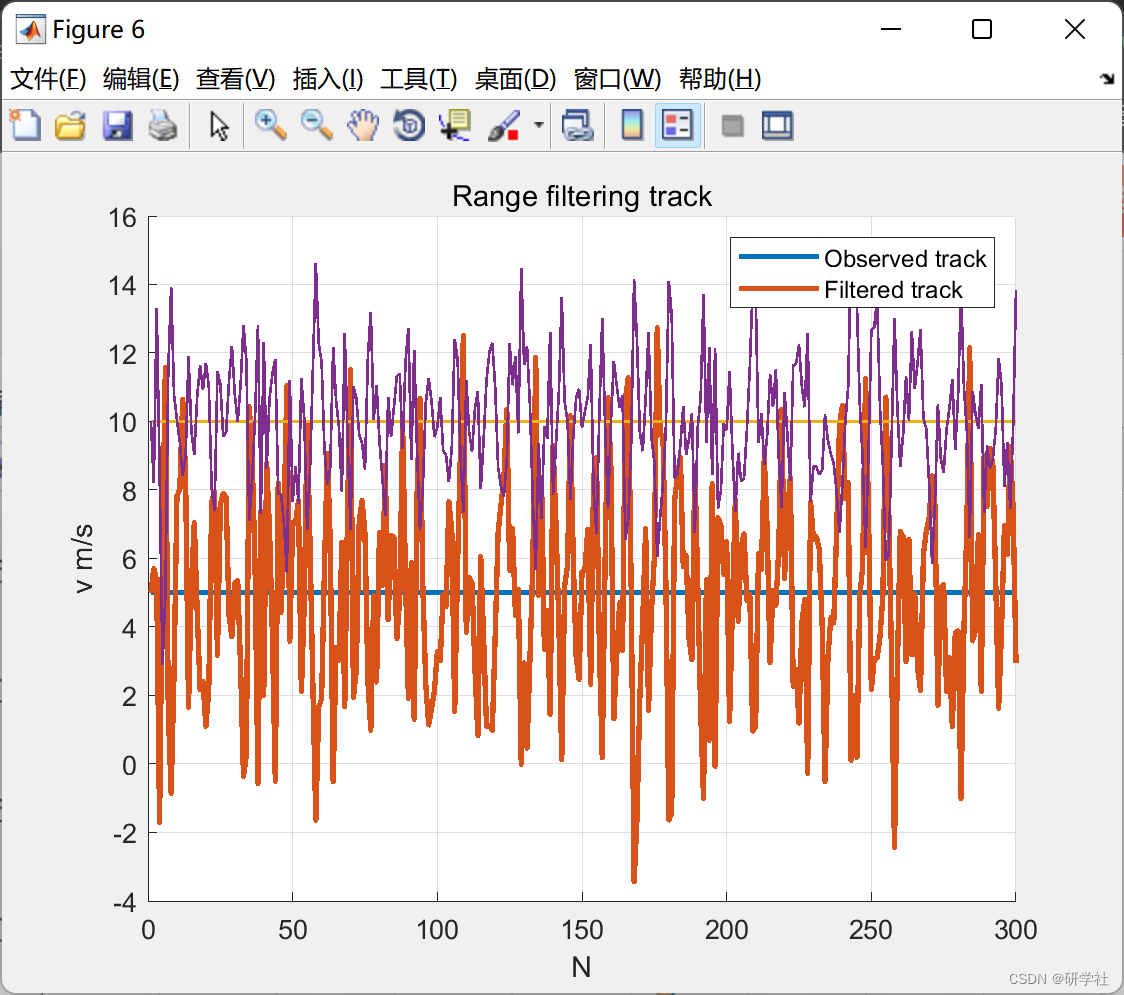
plot(X_real(2,:),'LineWidth',2);
plot(X_update(2,:),'LineWidth',2);

plot(X_real(4,:),'LineWidth',1);
plot(X_update(4,:),'LineWidth',1);
xlabel('N');ylabel('v m/s');legend('Observed track','Filtered track');
title('Range filtering track')

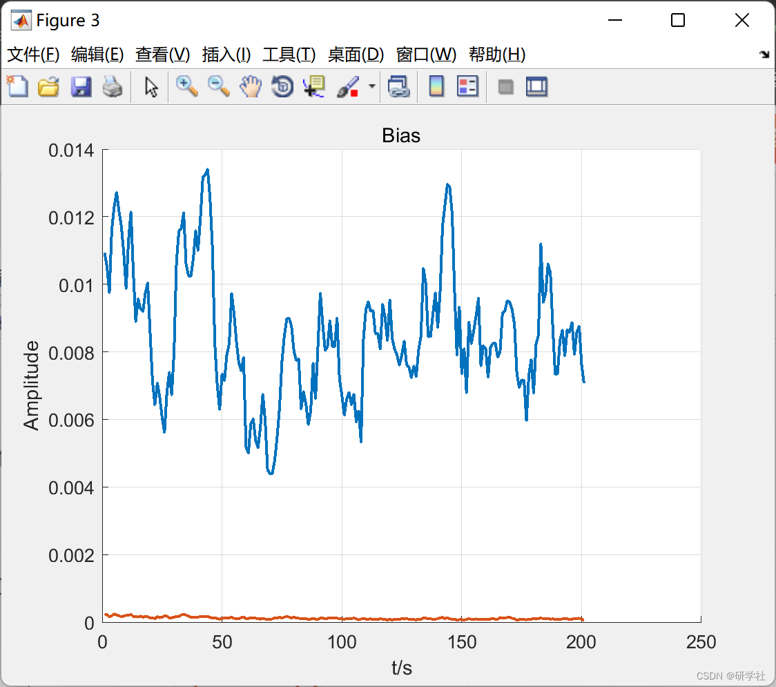
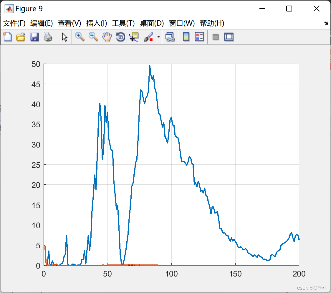
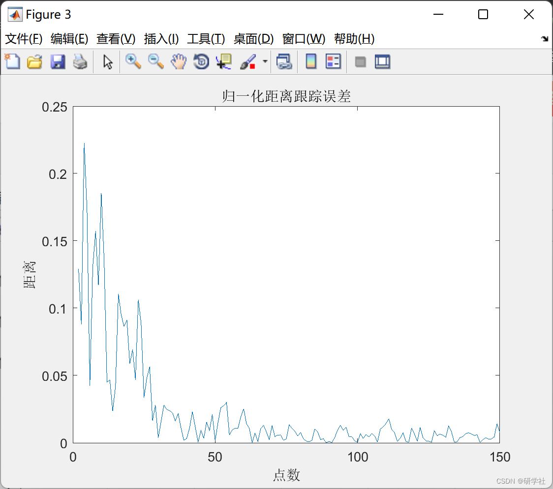
figure;grid on;
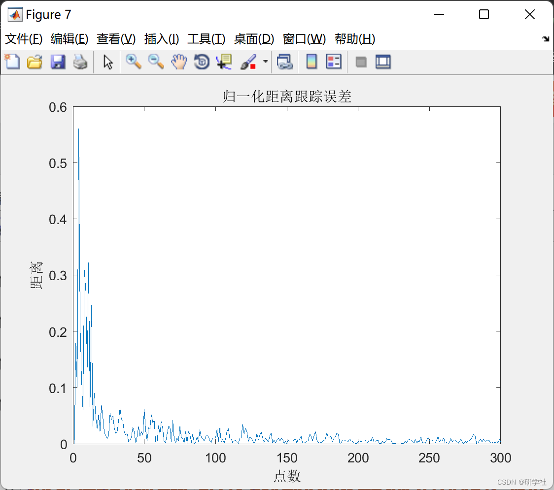
plot(abs(X_update(1,:)-X(1,:))./X(1,:));
title('归一化距离跟踪误差');xlabel('点数');ylabel('距离');
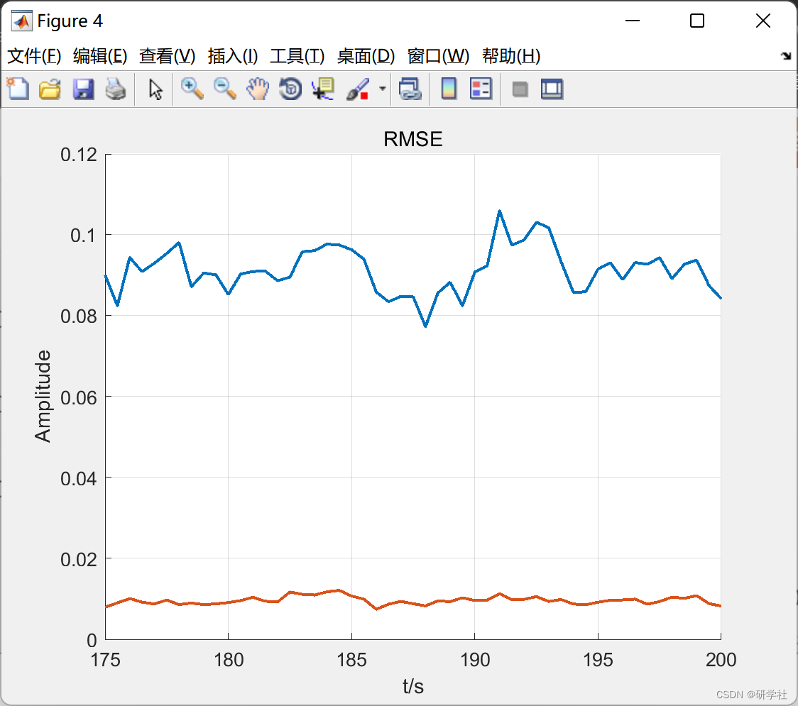
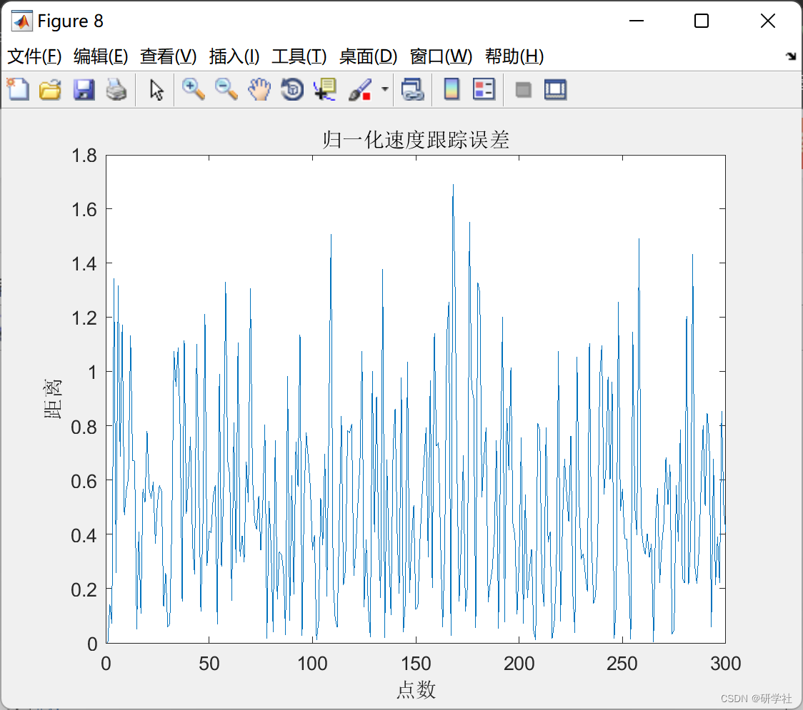
figure;grid on;
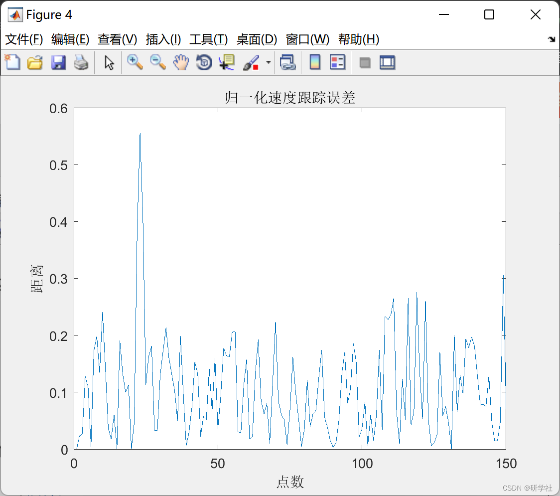
plot(abs(X_update(2,:)-X(2,:))./X(2,:));
title('归一化速度跟踪误差');xlabel('点数');ylabel('距离');

🎉3 参考文献

部分理论来源于网络，如有侵权请联系删除。

[1]刘欣欣,周传睿,姚元,伍光新,邢文革.面向多用户相控阵雷达通信的宽带波束赋形研究（英文）[J].现代雷达,2022,44(08):62-68.DOI:10.16592/j.cnki.1004-7859.2022.08.010.

[2]李国琳,郭文彬.雷达通信一体化波形设计综述[J].移动通信,2022,46(05):38-44.

🌈4 Matlab代码实现