Diffusion扩散模型简述 + 代码demo

FakeOccupational

已于 2023-07-26 10:57:36 修改

阅读量1w

点赞数 23

分类专栏：深度学习文章标签：概率论算法

于 2022-06-01 10:00:00 首次发布

本文链接：https://blog.csdn.net/ResumeProject/article/details/125017980

版权

深度学习专栏收录该内容

161 篇文章 16 订阅

订阅专栏

与GAN FLOW VAE类似扩散模型是一种生成模型。

在这里插入图片描述

需要用到的概率事实：

条件概率
马尔科夫链的转移公式
高斯分布的KL散度公式
$KL(P,Q)=log\frac{\sigma_2}{\sigma_1}+\frac{\sigma^2+(\mu_1-\mu_2)^2}{2\sigma_2^2} -\frac12 { \tiny(其中P.Q为一维高斯分布)}$
重参数技巧(从特殊高斯分布中采样点时不可导，将采样过程变为从标准分布N(0,1)采样的结果常量Z再用 $\mu$ , $\sigma$ 变为目标高斯分布)

在这里插入图片描述

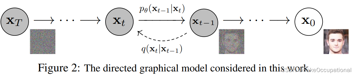
Diffusion

项目	描述 / $\cdot )$
$X_T$	各向同性的高斯分布 $N(X_T;0,I)$
$X_0$	训练数据集(的分布)

$\Leftarrow$ ：扩散过程，逐渐添加高斯噪声,有序到无序，熵增过程
$q(x_{1:T}|x_0):=\Pi_{t=1}^T q(x_t|x_{t-1}) \\ 其中q(x_t|x_{t-1}):=N(x_t;{\sqrt{1-\beta_t}x_{t-1}},\beta_t I)$
$\tiny \beta_t \in (0,1)可以如参考文献33设置为冲参数化的参数或直接设置为学习率一样的超参数\\所以正向过程是不含参数的。$

扩散过程的一个显著特性是，它允许以闭合形式在任意时间步t对xt进行采样：
$令a_t = 1-\beta_t \Downarrow \bar a_t=\Pi_{s=1}^t a_s \\ q(x_t|x_0)=N(x_t;\sqrt{\bar a_t}x_0,(1-\bar a_t)I)$

$上式的推导过程：\\ \tiny x_t= \sqrt{a_t}x_{t-1} + \sqrt{1-a_t}z_{t-1} \ ,在已知x_{t-1}时，确定x_t的高斯分布，其随机性由标准正太分布z_{t-1}提供\\ \quad = \sqrt{a_t}(\sqrt{a_{t-1}}x_{t-2} + \sqrt{1-a_{t-1}}z_{t-2}) + \sqrt{1-a_t}z_{t-1} \ \ \ 因为需要通过马尔科夫链获取x_t的分布 \\ \quad = \sqrt{a_t}\sqrt{a_{t-1}}x_{t-2} +(\sqrt{a_t} \sqrt{1-a_{t-1}}z_{t-2} + \sqrt{1-a_t}z_{t-1} )\ \ \ 因为需要通过马尔科夫链获取x_t的分布 \\ \quad = \sqrt{a_t}\sqrt{a_{t-1}}x_{t-2} +\sqrt {(\sqrt{a_t} \sqrt{1-a_{t-1}})^2 +(\sqrt{1-a_t} )^2 }z \ \ \ 标准正太分布方差的性质 \\ \quad =\sqrt{a_t a_{t-1}}x_{t-2} +\sqrt{1-a_ta_{t-1}}\bar z_{t-2} \ \ \qquad \qquad \quad \ \ \ \ \ \ \ \ \ \ \ \ \ \ \ \bar z为两个高斯分布的混合 \\ =\sqrt{\bar{a}_t}x_0+\sqrt{1-\bar{a}_t}z，\quad \quad 所以将上式写为q(x_t|x_0)=N(x_t;\sqrt{\bar a_t}x_0,(1-\bar a_t)I)$

unti-Diffusion

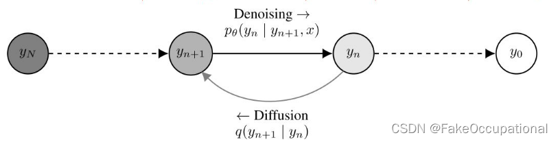
$\Rightarrow$ ：逆扩散过程(采样过程)，无序到有序，熵减过程
$联合分布p_{\theta}(x_{0:T}):=p(x_T)\Pi_{t=1}^T \ p_{\theta}(x_{t-1}|x_t) \\ 其中p_{\theta}(x_{t-1}|x_t):= N{(x_{t-1};\mu_{\theta}(x_t,t) ,\Sigma_{\theta}(x_t,t))}，\\ 即假设p_{\theta}(x_{t-1}|x_t)也为高斯分布,用网络拟合其中的系数\\ \mu_{\theta}(x_t,t) ,\Sigma_{\theta}(x_t,t)$
有了正向过程的分布，可以窥探逆向过程的分布，比如确定 $q(x_{t-1}| x_t,x_0)$ 的标准差和均值

$\tiny 根据贝叶斯定理转换P(A|B) 和 P(B|A)\\ q(x_{t-1}| x_t,x_0) = q(x_t|x_{t-1}.x_0)\frac{q(x_{t-1}|x_0)}{q(x_t|x_0)}\\ 正比于\propto exp(-\frac{1}{2}( \frac{(x_t-\sqrt{a_t}x_{t-1})^2}{\beta_t} + \frac{(x_{t-1}-\sqrt{\overline{a}_{t-1}}x_0)^2}{1-\bar{a}_{t-1}} -\frac{ (x_t - \sqrt{ \overline{a}_t}x_0)^2 }{1-\bar{a}_t} )) \\ = exp(-\frac{1}{2}( (\frac{a_t}{\beta_t }+\frac{1}{1-\bar a_{t-1}} )x_{t-1}^2 -(\frac{2\sqrt{a_t}}{\beta_t}x_t+\frac{2\sqrt{\overline a_t}}{1-\bar a_t}x_0)x_{t-1} +C(x_t,x_0) ))\\ 然后由二次函数得到-\frac{2a}{b}得到均值，和方差\\ 得到方差\bar \beta=\frac{1}{( \frac{a_t}{\beta_t }+\frac{1}{1-\bar a_{t-1}} )} = \frac{1-\bar a_{t-1}}{1-\bar a_t} \cdot \beta_t \\ 均值\bar{u}_t(x_t,x_0)=(\frac{\sqrt{a_t}}{\beta_t}x_t+\frac{\sqrt{\overline a_t}}{1-\bar{a_t}})/(\frac{\alpha_t}{\beta_t}+\frac{1}{1-\overline{\alpha}_{t-1}}) \\ =\frac{\sqrt{a_t}(1-\overline{a}_{t-1})}{1-\bar{a}_{t}}x_t+\frac{\sqrt{\overline{a}_{t-1}\beta_t}}{1-\bar a_t}x_0 \\ 参数重整化技巧\Downarrow x_t==\sqrt{\bar{a}_t}x_0+\sqrt{1-\bar{a}_t}z \\ \bar \mu_t=\frac{1}{\sqrt{a_t}}(x_t - \frac{\beta_t}{\sqrt{1-\overline{a}_t}}z_t)$

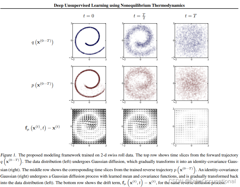
差值称为漂移量

loss函数

$p_{\theta}(x_0) \leq -logp_{\theta}(x_0) + D_{KL}(q(x_{1:T}|x_0)|| p_{\theta}(x_{1:T}|x_0)) \ {\tiny \color{blue}D_{KL} \geq 0} \\ \quad = -log p_{\theta}(x_0) +E_{x1:T \sim q(x1:T |x_0)}[log\frac{q(x_{1:T}|x_0)}{p_{\theta}(x_{1:T}|x_0)}] {\color{blue} \tiny KL散度公式展开为对log\frac{q}{p}用 p均值加权 P用来表示样本的真实分布，q用来表示模型所预测的分布} \\ \quad = -log p_{\theta}(x_0) +E_{x1:T \sim q(x1:T |x_0)}[log\frac{q(x_{1:T}|x_0)}{p_{\theta}(x_{0:T})/p_{\theta}(x_0)}] \\ \quad = -log p_{\theta}(x_0) +E_{q}[log\frac{q(x_{1:T}|x_0)}{p_{\theta}(x_{0:T})/p_{\theta}(x_0)}+logp_{\theta}(x_0)] \\ \quad = -log p_{\theta}(x_0) +E_{q}[log\frac{q(x_{1:T}|x_0)}{p_{\theta}(x_{0:T})/p_{\theta}(x_0)}] +logp_{\theta}(x_0) {\color{blue} \tiny +logp_{\theta}(x_0) 不受变量q加权的影响，直接移出来}\\ \quad =E_{q}[log\frac{q(x_{1:T}|x_0)}{p_{\theta}(x_{0:T})/p_{\theta}(x_0)}] {\color{blue} \tiny 至此得到了log似然函数的上界}\\$
$p_{\theta}(x_0)写成交叉熵的形式 \\ L = E_{q(x_0)}[-log p_{\theta}(x_0)] \\ \leq E_{q(x_0:T)}[log\frac{q(x_{1:T}|x_0)}{p_{\theta}(x_{0:T})}] {\color{blue} \tiny 将刚才计算的结果带入} \\ = E_{q(x_0:T)}[log\frac{ \Pi_{t=1}^{T} q(x_t|x_{t-1}) }{ p_{\theta}(x_{T}) \Pi_{t=1}^{T} p_{\theta}(x_{t-1}|x_{t}) } ] {\color{blue} \tiny 展开，上下类似，只不过一个时q扩散,一个是p逆扩散}\\ = E_{ q(x_0:T)}[ -log p_{\theta}(x_T)+\sum_{t=1}^T log\frac{ q(x_t|x_{t-1}) }{ p_{\theta}(x_{t-1}|x_{t}) } ] {\color{blue} \tiny } \\ = E_{ q(x_0:T)}[ -log p_{\theta}(x_T)+\sum_{t=2}^T log\frac{ q(x_t|x_{t-1}) }{ p_{\theta}(x_{t-1}|x_{t}) } {\color{blue} \tiny }+ log\frac{ q(x_t|x_{0}) }{ p_{\theta}(x_{0}|x_{t}) } ] {\color{blue} \tiny 取出其中的一项 } \\ {\tiny q(x_t|x_{t-1})= q(x_t|x_{t-1},x_0) \Downarrow = \frac{q(x_{t-1}|x_t,x_0)q(x_t|x_0)}{ q(x_{t-1}|x_0)} } \\ = E_{ q(x_0:T)}[ -log p_{\theta}(x_T)+\sum_{t=2}^T log\frac{ \frac{q(x_{t-1}|x_t,x_0)q(x_t|x_0)}{ q(x_{t-1}|x_0)} }{ p_{\theta}(x_{t-1}|x_{t}) } {\color{blue} \tiny }+ log\frac{ q(x_t|x_{0}) }{ p_{\theta}(x_{0}|x_{t}) } ] {\color{blue} \tiny }\\ = E_{ q(x_0:T)}[ -log p_{\theta}(x_T)+\sum_{t=2}^T log \frac{q(x_{t-1}|x_t,x_0)}{p_{\theta}(x_{t-1}|x_{t}) }\cdot \frac{q(x_t|x_0)}{ q(x_{t-1}|x_0)} {\color{blue} \tiny }+ log\frac{ q(x_t|x_{0}) }{ p_{\theta}(x_{0}|x_{t}) } ] {\color{blue} \tiny }\\ = E_{ q(x_0:T)}[ -log p_{\theta}(x_T)+\sum_{t=2}^T log \frac{q(x_{t-1}|x_t,x_0)}{p_{\theta}(x_{t-1}|x_{t}) }+\sum_{t=2}^T log\frac{q(x_t|x_0)}{ q(x_{t-1}|x_0)} {\color{blue} \tiny }+ log\frac{ q(x_t|x_{0}) }{ p_{\theta}(x_{0}|x_{t}) } ] {\color{blue} \tiny }\\ = E_{ q(x_0:T)}[ -log p_{\theta}(x_T)+\sum_{t=2}^T log \frac{q(x_{t-1}|x_t,x_0)}{p_{\theta}(x_{t-1}|x_{t}) }+log(\Pi_{t=2}^T \frac{q(x_t|x_0)}{ q(x_{t-1}|x_0)} ) {\color{blue} \tiny }+ log\frac{ q(x_t|x_{0}) }{ p_{\theta}(x_{0}|x_{t}) } ] {\color{blue} \tiny }\\ = E_{ q(x_0:T)}[ -log p_{\theta}(x_T)+\sum_{t=2}^T log \frac{q(x_{t-1}|x_t,x_0)}{p_{\theta}(x_{t-1}|x_{t}) }+log( \frac{q(x_T|x_0)}{ q(x_{1}|x_0)} ) {\color{blue} \tiny }+ log\frac{ q(x_t|x_{0}) }{ p_{\theta}(x_{0}|x_{t}) } ] {\color{blue} \tiny }\\ = E_{ q(x_0:T)}[ logq(x_T|x_0)-log p_{\theta}(x_T)+\sum_{t=2}^T log \frac{q(x_{t-1}|x_t,x_0)}{p_{\theta}(x_{t-1}|x_{t}) }+log( -{ q(x_{1}|x_0)} ) {\color{blue} \tiny } ] {\color{blue} \tiny }\\ = E_{ q(x_0:T)}[ {\color{blue}logq(x_T|x_0)-log p_{\theta}(x_T)}+ {\color{red}\sum_{t=2}^T log \frac{q(x_{t-1}|x_t,x_0)}{p_{\theta}(x_{t-1}|x_{t}) } }+log( -{ q(x_{1}|x_0)} ) {\color{blue} \tiny } ] {\color{blue} \tiny }\\ = E_{ q}[ {\color{blue}DKL（q(x_T|x_0)||p_{\theta}(x_T)）}+ {\color{red}\sum_{t=2}^T DKL（ {q(x_{t-1}|x_t,x_0)} || {p_{\theta}(x_{t-1}|x_{t}) } ）}+log( -{ q(x_{1}|x_0)} ) {\color{blue} \tiny } ] {\color{blue} \tiny }\\ \\ \Downarrow \\ blue :\ 常量，red \ L_{t-1}, \ black :L_{t-1}且t=1$
$论文假设p_{\theta}(x_{t-1}|x_{t})的方差为与\beta相关的常数，可训练参数仅有均值,主要关注红色部分$
$\Downarrow KL(P,Q)=log\frac{\sigma_2}{\sigma_1}+\frac{\sigma^2+(\mu_1-\mu_2)^2}{2\sigma_2^2} -\frac12 { \tiny(其中P.Q为一维高斯分布)}\\ L_{t-1}=E_q[ \frac{(\mu_1-\mu_2)^2}{2\sigma_t^2} ]\\ L_{t-1}=E_q[ \frac{(\mu_t(x_t,x_o)-\mu_{\theta}(x_t,t))^2}{2\sigma_t^2} ]+C\\ L_{t-1}=E_q[ \frac{(\mu_t(x_t,x_o)-\mu_{\theta}(x_t,t))^2}{2\sigma_t^2} ]+C\\ 其中\bar u_t逆行过程的均值，之前推导过,$

$L(\theta):=E_{t,x_0,\varepsilon} [|| \varepsilon -\varepsilon_{\theta}(\sqrt{\overline a_t},+ \sqrt{1-\overline a_t }\varepsilon,t))||^2] \\ L(\theta):=E_{t,x_0,\varepsilon} [|| \varepsilon -model_{\theta}( \overline a_t,\varepsilon,t))||^2]$

代码

# https://github.com/yangqy1110/Diffusion-Models/blob/main/Diffusion%20Model.ipynb
import  matplotlib.pyplot as plt
import numpy as np
from sklearn.datasets import make_s_curve
import torch

# TODO 实验数据
s_curve , _  = make_s_curve(10**4 , noise = 0.1)
s_curve = s_curve[:,[0,2] ]/10.0

print("shape of moons :",np.shape(s_curve))

data = s_curve.T

fig,ax = plt.subplots()
ax.scatter(*data ,color='red',edgecolor='white')
ax.axis('off')
plt.show()
dataset = torch.Tensor(s_curve).float() # shape of moons : (10000, 2)

# TODO 确定超参数的值
num_steps = 100 # 可以由beta alpha 分布 均值 标准差 进行估算

# 学习的超参数 动态的在（0，1）之间逐渐增大
betas = torch.linspace(-6,6,num_steps)
betas = torch.sigmoid(betas)* (0.5e-2 - 1e-5) + 1e-5

# 计算 alpha , alpha_prod , alpha_prod_previous , alpha_bar_sqrt 等变量的值
alphas = 1 - betas
alphas_prod = torch.cumprod( alphas ,dim=0 ) # 累积连乘  https://pytorch.org/docs/stable/generated/torch.cumprod.html
alphas_prod_p = torch.cat([torch.tensor([1]).float() ,alphas_prod[:-1]],0) # p means previous
alphas_bar_sqrt = torch.sqrt(alphas_prod)
one_minus_alphas_bar_log = torch.log(1-alphas_prod)
one_minus_alphas_bar_sqrt = torch.sqrt(1-alphas_prod)

assert  alphas_prod.shape == alphas_prod.shape == alphas_prod_p.shape \
        == alphas_bar_sqrt.shape == one_minus_alphas_bar_log.shape \
        == one_minus_alphas_bar_sqrt.shape
print("all the same shape:",betas.shape)  #


# TODO 确定扩散过程中任意时刻的采样值
def q_x(x_0 ,t):
    noise = torch.randn_like(x_0) # noise 是从正太分布中生成的随机噪声
    alphas_t = alphas_bar_sqrt[t] ## 均值 \sqrt{\bar \alpha_t}
    alphas_l_m_t = one_minus_alphas_bar_sqrt[t] ## 标准差  \sqrt{ 1 - \bar \alpha_t}
    # alphas_t = extract(alphas_bar_sqrt , t, x_0) # 得到sqrt(alphas_bar[t]) ,x_0的作用是传入shape
    # alphas_l_m_t = extract(one_minus_alphas_bar_sqrt , t, x_0) # 得到sqrt(1-alphas_bart[t])
    return (alphas_t * x_0 + alphas_l_m_t * noise)

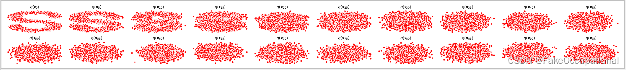
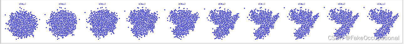
# TODO 演示原始数据分布加噪100步后的效果
num_shows = 20
fig , axs = plt.subplots(2,10,figsize=(28,3))
plt.rc('text',color='blue')
# 共有10000个点，每个点包含两个坐标
# 生成100步以内每隔5步加噪声后的图像
for i in range(num_shows):
    j = i // 10
    k = i % 10
    t = i*num_steps//num_shows # t=i*5
    q_i = q_x(dataset ,torch.tensor( [t] )) # 使用刚才定义的扩散函数，生成t时刻的采样数据  x_0为dataset
    axs[j,k].scatter(q_i[:,0],q_i[:,1],color='red',edgecolor='white')

    axs[j,k].set_axis_off()
    axs[j,k].set_title('$q(\mathbf{x}_{'+str(i*num_steps//num_shows)+'})$')
plt.show()

# TODO 编写拟合逆扩散过程 高斯分布 的模型
# \varepsilon_\theta(x_0,t)
import torch
import torch.nn as nn
class MLPDiffusion(nn.Module):
    def __init__(self,n_steps,num_units=128):
        super(MLPDiffusion,self).__init__()
        self.linears = nn.ModuleList([
            nn.Linear(2,num_units),
            nn.ReLU(),
            nn.Linear(num_units,num_units),
            nn.ReLU(),
            nn.Linear(num_units, num_units),
            nn.ReLU(),
            nn.Linear(num_units, 2),]

        )
        self.step_embeddings = nn.ModuleList([
            nn.Embedding(n_steps,num_units),
            nn.Embedding(n_steps, num_units),
            nn.Embedding(n_steps, num_units)
        ])
    def forward(self,x,t):
        for idx,embedding_layer in enumerate(self.step_embeddings):
            t_embedding = embedding_layer(t)
            x = self.linears[2*idx](x)
            x += t_embedding
            x = self.linears[2*idx +1](x)

        x = self.linears[-1](x)
        return x

# TODO loss　使用最简单的　loss
def diffusion_loss_fn(model,x_0,alphas_bar_sqrt,one_minus_alphas_bar_sqrt,n_steps):# n_steps 用于随机生成t
    '''对任意时刻t进行采样计算loss'''
    batch_size = x_0.shape[0]

    # 随机采样一个时刻t,为了体检训练效率，需确保t不重复
    # weights = torch.ones(n_steps).expand(batch_size,-1)
    # t = torch.multinomial(weights,num_samples=1,replacement=False) # [barch_size, 1]
    t = torch.randint(0,n_steps,size=(batch_size//2,)) # 先生成一半
    t = torch.cat([t,n_steps-1-t],dim=0) # 【batchsize,1】
    t = t.unsqueeze(-1)# batchsieze
    # print(t.shape)

    # x0的系数
    a = alphas_bar_sqrt[t]
    # 生成的随机噪音eps
    e = torch.randn_like(x_0)
    # eps的系数
    aml = one_minus_alphas_bar_sqrt[t]
    # 构造模型的输入
    x = x_0* a + e *aml
    # 送入模型，得到t时刻的随机噪声预测值
    output = model(x,t.squeeze(-1))


    # 与真实噪声一起计算误差，求平均值
    return (e-output).square().mean()


# TODO 编写逆扩散采样函数（inference过程）
def p_sample_loop(model ,shape ,n_steps,betas ,one_minus_alphas_bar_sqrt):
    '''从x[T]恢复x[T-1],x[T-2],……，x[0]'''

    cur_x = torch.randn(shape)
    x_seq = [cur_x]
    for i in reversed(range(n_steps)):
        cur_x = p_sample(model,cur_x, i ,betas,one_minus_alphas_bar_sqrt)
        x_seq.append(cur_x)
    return x_seq

def p_sample(model,x,t,betas,one_minus_alphas_bar_sqrt):
    '''从x[T]采样时刻t的重构值'''
    t = torch.tensor(t)
    coeff = betas[t] / one_minus_alphas_bar_sqrt[t]
    eps_theta = model(x,t)
    mean = (1/(1-betas[t]).sqrt())*(x-(coeff*eps_theta)) # 之前写错了：mean = (1/(1-betas[t].sqrt()) * (x-(coeff * eps_theta)))
    z = torch.randn_like(x)
    sigma_t = betas[t].sqrt()
    sample = mean + sigma_t * z
    return (sample)



# TODO 模型的训练
seed = 1234
class EMA():
    '''构建一个参数平滑器'''
    def __init__(self,mu = 0.01):
        self.mu =mu
        self.shadow = {}
    def register(self,name,val):
        self.shadow[name] = val.clone()

    def __call__(self, name, x): # call函数？
        assert name in self.shadow
        new_average = self.mu * x +(1.0 -self.mu) * self.shadow[name]
        self.shadow[name] = new_average.clone()
        return new_average

print('Training model ……')
'''
'''
batch_size = 128
dataloader = torch.utils.data.DataLoader(dataset,batch_size=batch_size,shuffle = True)
num_epoch = 4000
plt.rc('text',color='blue')

model = MLPDiffusion(num_steps) # 输出维度是2 输入是x 和 step
optimizer = torch.optim.Adam(model.parameters(),lr = 1e-3)

for t in range(num_epoch):
    for idx,batch_x in enumerate(dataloader):
        loss = diffusion_loss_fn(model,batch_x,alphas_bar_sqrt,one_minus_alphas_bar_sqrt,num_steps)
        optimizer.zero_grad()
        loss.backward()
        torch.nn.utils.clip_grad_norm(model.parameters(),1.) # 
        optimizer.step()
        # for name ,param in model.named_parameters():
        #   if params.requires_grad:
        #       param.data = ems(name,param.data)

    # print loss
    if (t% 100 == 0):
        print(loss)
        x_seq = p_sample_loop(model,dataset.shape,num_steps,betas,one_minus_alphas_bar_sqrt)# 共有100个元素

        fig ,axs = plt.subplots(1,10,figsize=(28,3))
        for i in range(1,11):
            cur_x = x_seq[i*10].detach()
            axs[i-1].scatter(cur_x[:,0],cur_x[:,1],color='red',edgecolor='white');
            axs[i-1].set_axis_off()
            axs[i-1].set_title('$q(\mathbf{x}_{'+str(i*10)+'})$')

基于扩散概率模型 (Diffusion Probabilistic Model ) 的音频生成模型
 添加链接描述
 https://www.jianshu.com/p/8b120d1881c1
(另辟蹊径—Denoising Diffusion Probabilistic 一种从噪音中剥离出图像/音频的模型)
在这里插入图片描述

paper Diffusion Models Beat GANs on Image Synthesis

disco-diffusion

disco difussion repo：https://github.com/alembics/disco-diffusion
openai guided diffusion https://github.com/openai/guided-diffusion

在colab上运行的视频
 github- docker - disco-diffusion

docker-本地运行版本
 https://github.com/MohamadZeina/Disco_Diffusion_Local
实现中先使用了clip进行了连接文本和图像

https://github.com/afiaka87/clip-guided-diffusion

哈哈

实验结果

在这里插入图片描述

额，好像没有跑回到S
注：昨天发现收到了一条评论(不知道是ta删除了还是其他原因，没有在下边的列表展示出来，感谢评论所指出的问题)
按照你的代码训了多次，找到问题了。代码本身没有问题。num_steps超参数给的太大了，因为这个数据很简单，所以加噪声到第四五次的

FakeOccupational

关注

23
点赞
踩
145

收藏

觉得还不错? 一键收藏
18
评论
Diffusion扩散模型简述 + 代码demo

扩散模型是一种生成模型GAN FLOW VAE需要用到的概率事实：条件概率马尔科夫链的转移公式高斯分布的KL散度公式KL(P,Q)=logσ2σ1+σ2+(μ1−μ2)22σ22−12(其中P.Q为一维高斯分布) KL(P,Q)=log\frac{\sigma_2}{\sigma_1}+\frac{\sigma^2+(\mu_1-\mu_2)^2}{2\sigma_2^2} -\frac12 { \tiny(其中P.Q为一维高斯分布)}KL(P,Q)=logσ1σ2+2σ22σ2+(μ
复制链接

扫一扫