


Laplacian Regularization
In Least Square learning methods, we calculate the Euclidean distance between sample points to find a classifier plane. However, here we calculate the minimum distance along the manifold of points and based on which we find a classifier plane.
In semi-supervised learning applications, we assume that the inputs
x
must locate in some manifold and the outputs
Take the Gaussian kernal function for example:
There are unlabeled samples {xi}n+n′i=n+1 that also be utilized:
In order to make all of the samples (labeled and unlabeled) have local similarity, it is necessary to add a constraint condition:
whose first two terms relate to the ℓ2 regularized least square learning and last term is the regularized term relates to semi-supervised learning ( Laplacian Regularization). v≥0 is a parameter to tune the smoothness of the manifold. Wi,i′≥0 is the similarity between xi and xi′ . Not familiar with similarity? Refer to:
Then how to solve the optimization problem? By the diagonal matrix
D
, whose elements are sums of row elements of
n=200; a=linspace(0,pi,n/2);
u=-10*[cos(a)+0.5 cos(a)-0.5]'+randn(n,1);
v=10*[sin(a) -sin(a)]'+randn(n,1);
x=[u v]; y=zeros(n,1); y(1)=1; y(n)=-1;
x2=sum(x.^2,2); hh=2*1^2;
k=exp(-(repmat(x2,1,n)+repmat(x2',n,1)-2*x*(x'))/hh);
w=k;
t=(k^2+1*eye(n)+10*k*(diag(sum(w))-w)*k)\(k*y);

m=100; X=linspace(-20,20,m)';X2=X.^2;
U=exp(-(repmat(u.^2,1,m)+repmat(X2',n,1)-2*u*(X'))/hh);
V=exp(-(repmat(v.^2,1,m)+repmat(X2',n,1)-2*v*(X'))/hh);
figure(1); clf; hold on; axis([-20 20 -20 20]);
colormap([1 0.7 1; 0.7 1 1]);
contourf(X,X,sign(V'*(U.*repmat(t,1,m))));
plot(x(y==1,1),x(y==1,2),'bo');
plot(x(y==-1,1),x(y==-1,2),'rx');
plot(x(y==0,1),x(y==0,2),'k.');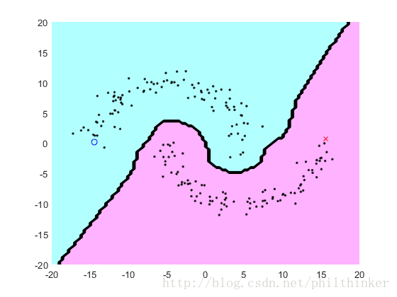


 1299
1299

 被折叠的 条评论
为什么被折叠?
被折叠的 条评论
为什么被折叠?
 到【灌水乐园】发言


