MIT | 数据分析、信号处理和机器学习中的矩阵方法 笔记系列: Lecture 7 Eckart-Young: The Closest Rank k Matrix to A

本系列为MIT Gilbert Strang教授的"数据分析、信号处理和机器学习中的矩阵方法"的学习笔记。

• Gilbert Strang & Sarah Hansen | Sprint 2018
• 18.065: Matrix Methods in Data Analysis, Signal Processing, and Machine Learning
• 视频网址: https://ocw.mit.edu/courses/18-065-matrix-methods-in-data-analysis-signal-processing-and-machine-learning-spring-2018/
• 关注 下面的公众号，回复“ 矩阵方法 ”，即可获取 本系列完整的pdf笔记文件~

---

内容在CSDN、知乎和微信公众号同步更新

• CSDN博客
• 知乎
• 微信公众号
• qq邮箱: 981591477

• Markdown源文件暂未开源，如有需要可联系邮箱
• 笔记难免存在问题，欢迎联系邮箱指正

---

Lecture 0: Course Introduction

Lecture 1 The Column Space of $A$ Contains All Vectors $Ax$

Lecture 2 Multiplying and Factoring Matrices

Lecture 3 Orthonormal Columns in $Q$ Give $Q^{\prime }Q=I$

Lecture 4 Eigenvalues and Eigenvectors

Lecture 5 Positive Definite and Semidefinite Matrices

Lecture 6 Singular Value Decomposition (SVD)

Lecture 7 Eckart-Young: The Closest Rank $k$ Matrix to $A$

Lecture 8 Norms of Vectors and Matrices

Lecture 9 Four Ways to Solve Least Squares Problems

Lecture 10 Survey of Difficulties with $Ax=b$

Lecture 11 Minimizing ||x|| Subject to $Ax=b$

Lecture 12 Computing Eigenvalues and Singular Values

Lecture 13 Randomized Matrix Multiplication

Lecture 14 Low Rank Changes in $A$ and Its Inverse

Lecture 15 Matrices $A(t)$ Depending on $t$, Derivative = $dA/dt$

Lecture 16 Derivatives of Inverse and Singular Values

Lecture 17 Rapidly Decreasing Singular Values

Lecture 18 Counting Parameters in SVD, LU, QR, Saddle Points

Lecture 19 Saddle Points Continued, Maxmin Principle

Lecture 20 Definitions and Inequalities

Lecture 21 Minimizing a Function Step by Step

Lecture 22 Gradient Descent: Downhill to a Minimum

Lecture 23 Accelerating Gradient Descent (Use Momentum)

Lecture 24 Linear Programming and Two-Person Games

Lecture 25 Stochastic Gradient Descent

Lecture 26 Structure of Neural Nets for Deep Learning

Lecture 27 Backpropagation: Find Partial Derivatives

Lecture 28 Computing in Class [No video available]

Lecture 29 Computing in Class (cont.) [No video available]

Lecture 30 Completing a Rank-One Matrix, Circulants!

Lecture 31 Eigenvectors of Circulant Matrices: Fourier Matrix

Lecture 32 ImageNet is a Convolutional Neural Network (CNN), The Convolution Rule

Lecture 33 Neural Nets and the Learning Function

Lecture 34 Distance Matrices, Procrustes Problem

Lecture 35 Finding Clusters in Graphs

Lecture 36 Alan Edelman and Julia Language

---

---

Lecture 7 Eckart-Young: The Closest Rank k Matrix to A

This is a pretty key lecture

• about principal component analysis (PCA)
• a major tool in understanding a matrix of data

7.1 Review SVD & Propose Eckart-Young Theorem

• $A=U\Sigma V^T={\sigma }_1{u}_1{v}_1^T+...+{\sigma }_r{u}_r{v}_r^T$

  • any matrix $A$ could be broken into r rank 1 pieces

  • $r$: the rank of the matrix $A$

  • $u$ and $r$: orthonomal

  • how to get important information:

    ❌ (People say, in machine learning, if you learned all of the training data, you have not learned anything $\Rightarrow$ just copy and overfitting)

    🚩 The whole point of DNN and the process of ML is to learn the import facts about the data

    🚩 The most basic stage of that: TOP (Largest) k singular values $\Rightarrow$ $A_k=U_k{\Sigma }_k{V}_k^T={\sigma }_1{u}_1{v}_1^T+...+{\sigma }_k{u}_k{v}_k^T$

    ✅ One Theorem here: $A_k$ using the first k pieces of the SVD is the best approximation to $A$ of rank $k$ $\Rightarrow$ 🚩 This really says why SVD is perfect

    ✅ More precisely Definition: (Eckart-Young Theorem) If B has rank k, then $\Vert A-B\Vert$ $\ge$ $\Vert A-A_k\Vert$ $\Rightarrow$ a pretty straightform beautiful fact

下面要解决的问题：

1. 范数：定理中的$\Vert \cdot \Vert$的含义
2. 证明该定理

7.2 Norm of Matrix

本节课介绍的范数的特点: can be comupted by their singular values

• Pre: Norm of Vectors

• $\Vert v{\Vert }_2$: just the regular lenght of vector $\sqrt{|v_1{|}^2+|v_2{|}^2+...+|v_n{|}^2}$

  🚩 historically goes back to Gauss $\Rightarrow$ the least squares

  🚩 the results would have lot of little components (平方后do not hurt much)

• $\Vert v{\Vert }_1$ = $|v_1|+...+|v_n|$ $\Rightarrow$ 🚩 getting more and more important & special

  🚩 🚩 when you minimize some function using the $L_1$ norm

  ▪ 🚩 tend to be sparse $\Rightarrow$ mostly zero components

  ✅ One advantage of the “sparse” : you can understand what its components are $\Rightarrow$ 如果一个result有很多small components, 解释起来就会很困难($L_2$); 反之($L_1$)，则易于解释

• $\Vert v{\Vert }_{\infty }$ = max $|v_i|$

• The property of the norm:

  🚩 homogeneous : $\Vert CV\Vert =|C|\Vert V\Vert$ $\Rightarrow$ If you double the vector, you should double the norm

  ✅ triangle inequality : $\Vert V+W\Vert \le \Vert V\Vert +\Vert W\Vert$ $\Rightarrow$ add the norm of V and W, you get more than the straight norm along the hypotenuse hypotenuse 斜边 $\Rightarrow$

  🚩 上述properties 同样适用于Matrix Norm $\downarrow$

• 矩阵范数1: $L_2$ Norm

  • The largst singular value
  • $\Vert A{\Vert }_2={\sigma }_1$
  • Property 1: homogeneous $\Rightarrow$ $\Vert 2A{\Vert }_2=2{\sigma }_1$
  • Property 2: Triangle inequality $\Rightarrow$ The largest singular value of $A+B$ $\le$ the largest singular value of A + the largest singular value of B

• 矩阵范数2：Frobenius norm $\Vert A{\Vert }_F=\sqrt{|a_{11}{|}^2+...+|a_{nm}{|}^2}$

  • just like the $L_2$ vector norm

• 矩阵范数3：Nuclear norm $\Vert A{\Vert }_{Nuclear}={\sigma }_1+{\sigma }_2+...+{\sigma }_r$

  • 考虑Netflix Competitions: It had movie preferences from many Netflix subscribers $\Rightarrow$ they give their ranking to a bunch of movies $\Rightarrow$ none of them had seen all the movies $\Rightarrow$ So, the matrix of rankings – the ranker and the matrix – is a bery big matrix $\Rightarrow$ but it got missing entries – if the ranker did not see the movie, 则无法ranking it

  • 那么 what is the idea about Netflix?

    ✅ what would the ranker have said about the post if he had not seen it, but have ranked several other movies

    🚩 The Nuclear Norm is the right one to minimize!

  • and MRI

• 对于以上三种Matrix Norm, the theorem: $A_k$ using the first k pieces of the SVD is the best approximation to $A$ of rank $k$ is ture

下节课将会对范数进行更加详细的介绍

7.3 About Eckart-Young theorem

没有证明该定理，但是举例说明了该定理的含义和适用范围

• The above 3 Matrix Norm 适用于该定理 (但并非all Matrix Norm)

• Why?

  • These 3 norms depend only on the singular values

    🚩 $\Vert A{\Vert }_2$ and $\Vert A{\Vert }_{Nuclear}$ obviously depends on singular values

  • Suppose $k=2$ $\Rightarrow$ looking among all rank 2 matrices

    ✅ and the matrix $\Sigma =\left[\begin{array}{cccc}4& 0& 0& 0\\ 0& 3& 0& 0\\ 0& 0& 2& 0\\ 0& 0& 0& 1\end{array}\right]$

    🚩 the best approximation of rank 2 ${\Sigma }_2=\left[\begin{array}{cccc}4& 0& 0& 0\\ 0& 3& 0& 0\\ 0& 0& 0& 0\\ 0& 0& 0& 0\end{array}\right]$

    ✅ and an exmple of $B=\left[\begin{array}{cccc}3.5& 3.5& 0& 0\\ 3.5& 3.5& 0& 0\\ 0& 0& 1.5& 1.5\\ 0& 0& 1.5& 1.5\end{array}\right]$ $\Rightarrow$ 一行两个3.5 (1.5) 是为了 keep low rank

  • 对于非对角阵 $A=U\Sigma V^T$

    ✅ What are the singular values of that matrix $A$? $\Rightarrow$ did not change! – 4,3,2,1 $\Rightarrow$ because $A=U\Sigma V^T$ is an SVD form and the diagonal contains diagonal values

    🚩 The problem is orthogonally invariant.

    ✅ These norms are not changed by orthogonal matrices $\Rightarrow$ $QA=QU\Sigma V^T=U^{\prime }\Sigma V^T$ (Orthogonal $\times$ Orthogonal is Orthogonal)

• These are the key math behind PCA

---

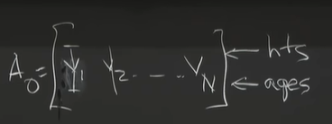
• An example: 研究身高和年龄的关系

  • (PCA Principal Component Analysis用于拟合可参考相关博客，如 https://xiaotaoguo.com/p/pca-model-fitting/)

  • data matrix $A_0$ (如下图)

  • 1st step: normalization (get the mean to zero) $\Rightarrow$ $A=A_0-[averag{e}_{h}eight;//averag{e}_{a}ges]$

    🚩 centered the data at $(0,0)$

  • How to looking for the best line to fit the data (in the data matrix)? (What is the best linear relationship?)

    ✅ here is PCA as a linear business (instead of unlinear deep learning method)

  • One way: use least squares (Gauss did it). $\Rightarrow$ 🚩 使用PCA和使用least squares的区别？

    🚩 In PCA, you are measuring perpendicular to the lineperpendicular 垂直 $\Rightarrow$ involve SVD / $\sigma$

    🚩 但 least square 则用的竖直距离 ($\Vert Ax-b{\Vert }^2$) $\Rightarrow$ $A^{T}A\hat{x}=A^{T}b$ (regression problem)

    🚩 Sample Covariance matrix $A{A}^T$

---

本节小结:

1. 给出了 One Theorem: $A_k$ using the first k pieces of the SVD is the best approximation to $A$ of rank $k$
2. 引入并介绍了 向量范数 和 矩阵范数 的概念
3. 根据范数的概念，详细说明了 上述定理的含义和应用范围
4. 根据上述定理， 引入了PCA ，举例说明了PCA和SVD在数据拟合上的应用