Ceres简介及示例（5）Bundle Adjustment

aworkholic

已于 2023-06-08 13:42:23 修改

阅读量1.2k

点赞数

分类专栏： # Ceres 数值优化文章标签：人工智能 ceres ba 捆集调整非线性优化

于 2023-04-02 22:19:14 首次发布

本文链接：https://blog.csdn.net/wanggao_1990/article/details/129686526

版权

Ceres 同时被 2 个专栏收录

11 篇文章

订阅专栏

数值优化

11 篇文章

订阅专栏

编写Ceres的主要原因之一是我们需要解决大规模的Bundle Adjustment问题。

给定一组测量的图像特征位置和对应关系，Bundle Adjustment的目标是找到使重投影误差最小的三维点位置和摄像机参数。

该优化问题通常表述为非线性最小二乘问题，其中误差为观测特征位置与相应三维点在摄像机图像平面上的投影差的L2范数的平方。Ceres广泛支持解决Bundle Adjustment问题。

1、BAL问题和数据集

在一个场景中，有多个三维空间点路标，相机在不同姿态下观测路标得到路标在图像中的像素坐标，最终需要优化相机的参数和路标的空间位置。例如下面

本例中使用problem-16-22106-pre.txt作为例子，该文件薪资中包含的相机模型和数据格式的详细信息可以在 Bundler主页和 BAL主页上找到。如下流图所示，空间中有两个相机 $C_{1}$ 和 $C_{2}$ ，有6个路标 $P_{1}$ 、 $P_{2}$ 、 $P_{3}$ 、 $P_{4}$ 、 $P_{5}$ 、 $P_{6}$ ，相机 $C_{1}$ 观测到前4个路标，相机 $C_{2}$ 观测到后4个路标，整个数据中就存在8个观测点。

相机模型
这里示例使用针孔相机模型，需要估计的参数有空间旋转 R，位移t，焦距f 和径向畸变系数k1, k2。空间中三维点投影到相机中的公式为：
$(世界坐标系到相机坐标系)\\ p = -P / P.z (归一化像平面的齐次坐标)\\ p' = f* r(p)*p (图像坐标系到像素坐标系)$
这里的 $P . z$ 是点P的z轴数据. 最后一个公式中 $r (p)$ 函数用于消除畸变操作：
$r(p) = 1.0 + k_1 * ||p||^2 + k_2 * ||p||^4 \\ 　　　　　　　= 1.0 +||p||^2( k_1 + k_2 * ||p||^2 )（用于计算）$

数据格式
ceres项目默认包含了文件，路径为 ceres-solver-1.14.0/dataproblem-16-22106-pre.txt。

<num_cameras> <num_points> <num_observations>
<camera_index_1> <point_index_1> <x_1> <y_1>
...
<camera_index_num_observations> <point_index_num_observations> <x_num_observations> <y_num_observations>
<camera_1>
...
<camera_num_cameras>
<point_1>
...
<point_num_points>

场景中含有16个相机，一共22106个路标，一个路标可以被多个相机观测到，如 0号路标被相机{0,1,2,7,12,13}观测到，且在相机0中的像素位置为{-385.99，387.12}，整个场景中共有83718个观测点。

// problem-16-22106-pre.txt
16 22106 83718
0 0     -3.859900e+02 3.871200e+02
1 0     -3.844000e+01 4.921200e+02
2 0     -6.679200e+02 1.231100e+02
7 0     -5.991800e+02 4.079300e+02
12 0     -7.204300e+02 3.143400e+02
13 0     -1.151300e+02 5.548999e+01
0 1     3.838800e+02 -1.529999e+01
1 1     5.597500e+02 -1.061500e+02

2、问题构建

2.1、定义投影误差模型

第一步通常是定义一个模板化的仿函数来计算重投影误差/残差。仿函数的结构类似于ExponentialResidual，因为每个图像观测都有一个该对象的实例。

注意：

相机内参模型有焦距f和畸变参数k1、k2给出，这里将fx和fy等同起来，另外模型中没有cx和cy，因为存储数据中已经去掉，计算不参与。
BAL数据在投影时假设投影平面在相机光心之后，与假设的小孔成像模型投影平面在相机光心之前相反，因此需要在投影之后乘以系数-1。

BAL问题中的每个残差都依赖于一个三维点和九个相机参数。定义摄像机的9个参数是:3个旋转作为罗德里格斯轴-角向量，3个平移，1个焦距，2个径向畸变。

// Templated pinhole camera model for used with Ceres.  The camera is
// parameterized using 9 parameters: 3 for rotation, 3 for translation, 1 for
// focal length and 2 for radial distortion. The principal point is not modeled
// (i.e. it is assumed be located at the image center).
struct SnavelyReprojectionError {
	// 读入两个参数，空间点在成像平面上的位置，并赋值。
  SnavelyReprojectionError(double observed_x, double observed_y)
      : observed_x(observed_x), observed_y(observed_y) {}

	// 重载操作符()
  template <typename T>
  bool operator()(const T* const camera,
                  const T* const point,
                  T* residuals) const {
    // camera[0,1,2] are the angle-axis rotation.
    T p[3];
    ceres::AngleAxisRotatePoint(camera, point, p);
    // camera[3,4,5] are the translation.
    p[0] += camera[3]; p[1] += camera[4]; p[2] += camera[5];

    // Compute the center of distortion. The sign change comes from
    // the camera model that Noah Snavely's Bundler assumes, whereby
    // the camera coordinate system has a negative z axis.
    T xp = - p[0] / p[2];
    T yp = - p[1] / p[2];

    // Apply second and fourth order radial distortion.
    const T& l1 = camera[7];
    const T& l2 = camera[8];
    T r2 = xp*xp + yp*yp;
    T distortion = 1.0 + r2  * (l1 + l2  * r2);

    // Compute final projected point position.
    const T& focal = camera[6];
    T predicted_x = focal * distortion * xp;
    T predicted_y = focal * distortion * yp;

    // The error is the difference between the predicted and observed position.
    residuals[0] = predicted_x - T(observed_x);
    residuals[1] = predicted_y - T(observed_y);
    return true;
  }

   // Factory to hide the construction of the CostFunction object from
   // the client code.
   static ceres::CostFunction* Create(const double observed_x,
                                      const double observed_y) {
     return (new ceres::AutoDiffCostFunction<SnavelyReprojectionError, 2, 9, 3>(
                 new SnavelyReprojectionError(observed_x, observed_y)));
   }

  double observed_x;
  double observed_y;
};

注意，与前面的例子不同，这是一个非平凡函数(non-trivial function)，计算它的解析雅可比矩阵有点麻烦。如果使用自动微分法就会容易很多。
函数AngleAxisRotatePoint()和其他操作旋转的函数可以在include/ceres/rotation.h中找到。

2.2、数据读取预处理

用BLAProblem类读取数据之后，可以调用Normalize函数对原始数据进行归一化，或通过Perturb函数给数据加上噪声。

  BALProblem bal_problem(filename, FLAGS_use_quaternions);

  if (!FLAGS_initial_ply.empty()) {
    bal_problem.WriteToPLYFile(FLAGS_initial_ply);
  }

  Problem problem;

  srand(FLAGS_random_seed);
  bal_problem.Normalize();
  bal_problem.Perturb(FLAGS_rotation_sigma,
                      FLAGS_translation_sigma,
                      FLAGS_point_sigma);

归一化是将所有路标点的中心置零，然后做一个合适尺度的缩放，这样能使优化过程中数值更稳定，防止在极端情况下处理很大或者很大偏移的BA问题。

2.3、问题构建

给定这个仿函数，bundle adjustment问题可以构造如下:

ceres::Problem problem;
for (int i = 0; i < bal_problem.num_observations(); ++i) {
  ceres::CostFunction* cost_function =
      SnavelyReprojectionError::Create(
           bal_problem.observations()[2 * i + 0],
           bal_problem.observations()[2 * i + 1]);
  problem.AddResidualBlock(cost_function,
                           nullptr /* squared loss */,
                           bal_problem.mutable_camera_for_observation(i),
                           bal_problem.mutable_point_for_observation(i));
}

注意，bundle adjustment的问题构造与曲线拟合的例子非常相似——每次观测都向目标函数中添加一项。

2.4、求解

因为这是一个大规模稀疏矩阵问题(至少对于DENSE_QR很大)，解决这个问题的一种方法是设置Solver::Options::linear_solver_type为SPARSE_NORMAL_CHOLESKY，并调用solve()
虽然这是一个合理的做法，bundle adjustment问题有一个特殊的稀疏结构，可以利用这个更有效地解决它们。Ceres为此任务提供了三个专门的求解器(统称为基于schur的求解器)。示例代码使用其中最简单的DENSE_SCHUR。

ceres::Solver::Options options;
options.linear_solver_type = ceres::DENSE_SCHUR;
options.minimizer_progress_to_stdout = true;
ceres::Solver::Summary summary;
ceres::Solve(options, &problem, &summary);
std::cout << summary.FullReport() << "\n";

可见问题搭建部分是相当简单的，如果要添加别的代价函数，整个流程也不会太多变化。使用DENSE_SCHUR会让Ceres先对路标进行Schur边缘化，以加速的方式解此问题。不过在Ceres中不能控制哪部分变量被边缘化，这是由求解器自动寻找并计算的。

3、结果

运行输出为

iter      cost      cost_change  |gradient|   |step|    tr_ratio  tr_radius  ls_iter  iter_time  total_time
   0  4.185660e+06    0.00e+00    2.16e+07   0.00e+00   0.00e+00  1.00e+04        0    7.09e-02    2.15e-01
   1  1.980525e+05    3.99e+06    5.34e+06   2.40e+03   9.60e-01  3.00e+04        1    3.15e-01    5.30e-01
   2  5.086543e+04    1.47e+05    2.11e+06   1.01e+03   8.22e-01  4.09e+04        1    2.93e-01    8.24e-01
   3  1.859667e+04    3.23e+04    2.87e+05   2.64e+02   9.85e-01  1.23e+05        1    2.92e-01    1.12e+00
   4  1.803857e+04    5.58e+02    2.69e+04   8.66e+01   9.93e-01  3.69e+05        1    2.96e-01    1.41e+00
   5  1.803391e+04    4.66e+00    3.11e+02   1.02e+01   1.00e+00  1.11e+06        1    2.91e-01    1.70e+00

Solver Summary (v 1.14.0-eigen-(3.3.7)-lapack-suitesparse-(5.4.0)-cxsparse-(3.1.9)-eigensparse-openmp-no_tbb-no_custom_blas)

                                     Original                  Reduced
Parameter blocks                        22122                    22122
Parameters                              66462                    66462
Residual blocks                         83718                    83718
Residuals                              167436                   167436

Minimizer                        TRUST_REGION

Sparse linear algebra library    SUITE_SPARSE
Trust region strategy     LEVENBERG_MARQUARDT

                                        Given                     Used
Linear solver                    SPARSE_SCHUR             SPARSE_SCHUR
Threads                                     1                        1
Linear solver ordering              AUTOMATIC                 22106,16
Schur structure                         2,3,9                    2,3,9

Cost:
Initial                          4.185660e+06
Final                            1.803391e+04
Change                           4.167626e+06

Minimizer iterations                        6
Successful steps                            6
Unsuccessful steps                          0

Time (in seconds):
Preprocessor                         0.144149

  Residual only evaluation           0.081206 (5)
  Jacobian & residual evaluation     0.333301 (6)
  Linear solver                      1.036461 (5)
Minimizer                            1.560524

Postprocessor                        0.003255
Total                                1.707929

Termination:                   NO_CONVERGENCE (Maximum number of iterations reached. Number of iterations: 5.)

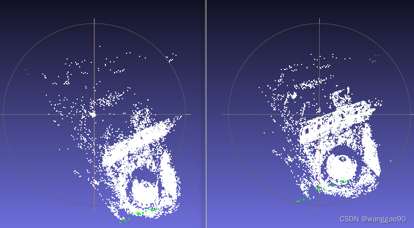
使用meshlab打开BA优化前后的ply文件如下，显然优化后的效果要更好。
在这里插入图片描述