Drug 2. 临床标志物之药物敏感性水平 (oncoPredict)

上期我们介绍了临床标志物之药物-基因关联预测，这期继续介绍药物敏感性水平的计算。

---

临床前生物标志物发现

这个脚本提供了一个如何在临床前生物标志物发现中控制一般药物敏感性水平 general levels of drug sensitivity (GLDS)的例子。

具体来说，这个脚本对GDSCv2数据应用glds函数来获得每个#drug-gene关联的p值和beta值。控制GLDS很重要，因为GLDS的变异性在癌细胞系中很明显，控制这种变异性可以促进癌症生物标志物的发现。

读取相关数据

读取GDSC更新的细胞系信息文件：Cell_Lines_Details.csv

读取药物反应数据文件：complete_matrix_output_GDSCv2.txt

读取以正确的顺序包含药物反应数据的颜色名，但删除了额外的标识符的文件：gdscv2_drugs.txt

读取GDSCv2更新泛癌突变数据集包括CNV和编码变体的文件：markerMat.txt

读取GDSC更新的药物相关性文件(来自大数据下载/所有筛选的化合物/化合物-注释)：screened_compunds_rel_8.2.csv

library(oncoPredict)
cellLineDetails <- read.csv("./oncoPredict-main/vignettes/Cell_Lines_Details.csv")
dim(cellLineDetails)
## [1] 1002   13
cm <- read.table("./oncoPredict-main/vignettes/complete_matrix_output_GDSCv2.txt",
    header = TRUE, row.names = 1)
newRows <- substring(rownames(cm), 8)  #Remove 'COSMIC'...keep the numbers after COSMIC.
indices <- match(as.numeric(newRows), as.vector(unlist(cellLineDetails[, 2])))  #Refer to the cell
newNames <- as.vector(unlist(cellLineDetails[, 1]))[indices]  #Reports the corresponding cell line names
rownames(cm) <- newNames
fix <- as.vector(unlist(read.table("./oncoPredict-main/vignettes/gdscv2_drugs.txt",
    header = TRUE)))
colnames(cm) <- as.vector(fix)
drugMat <- as.matrix(cm)  #Finally, set this object as the drugMat parameter. 
dim(drugMat)
## [1] 100 198
markerMat <- as.matrix(read.table("./oncoPredict-main/vignettes/markerMat.txt", header = TRUE,
    row.names = 1))
drugRelatedness <- read.csv("./oncoPredict-main/vignettes/screened_compunds_rel_8.2.csv")
drugRelatedness <- drugRelatedness[, c(3, 6)]

glds()函数计算药物敏感性

参数说明：

minMuts：可以计算p值所需的最小非零条目数；

additionalCovariateMatrix：包含在药物生物标志物关联模型中拟合的协变量的矩阵。

expression：表达数据的矩阵。rownames()是基因，colnames()是与药物gmat中相同的临床前样本(顺序也相同)。默认值为NULL。如果提供表达数据，将获得基因名。

threshold：确定相关系数。与被检查药物相关系数大于或等于该数值的药物将从阴性对照组中移除。默认值是0.7

glds(drugMat, drugRelatedness, markerMat, minMuts = 5, additionalCovariateMatrix = NULL,
    threshold = 0.7)

结果解读及可视化

获得的结果中生产是个文件分别naive的beta值和P值，还有glds的beta值和P值：

naiveBetas.csv

naivePs.csv

gldsBetas.csv

gldsPs.csv

并对结果数据进行可视化，由于gldsPs.csv里面并未找到敏感性药物，因此只做了naive的可视化分析。

library(reshape2)
library(ggplot2)
naiveBetas<-na.omit(read.csv("naiveBetas.csv"))
naiveBetas<-melt(naiveBetas,id.vars = "X",value.name="BetaVal",variable.name ="drug")
naivePs<-na.omit(read.csv("naivePs.csv"))
naivePs<-melt(naivePs,id.vars = "X",value.name="pVal",variable.name ="drug")
naive<-merge(naiveBetas,naivePs,by = c("X","drug"))

ggplot(naive[naive$pVal<0.05,],aes(x=drug,y=X))+ #热图绘制
  scale_color_gradientn(values = seq(0,1,0.2),colours = c('#6699CC','#FFFF99','#CC3333'))+
  theme_bw()+
  geom_point(aes(size=`pVal`,color=`BetaVal`))+
  theme(axis.text.x =element_text(angle =90,hjust =0.5,vjust = 0.5))+
  xlab(NULL) + ylab(NULL)+
  theme(panel.border = element_rect(fill=NA,color="black", size=1, linetype="solid"))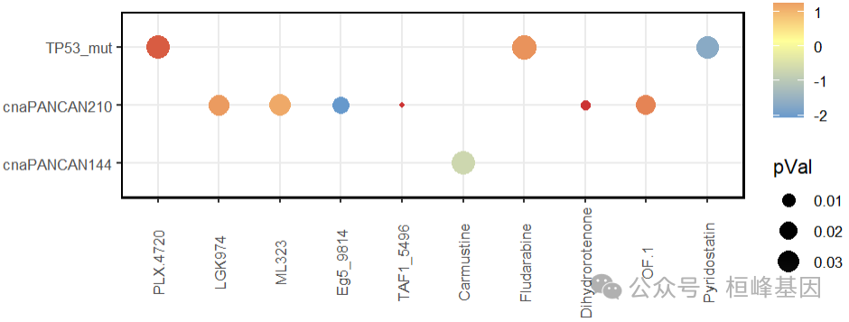

# geom_vline(xintercept=c(-3,3.5,8.5,11.5,15.5),size=.8)


gldsBetas<-na.omit(read.csv("gldsBetas.csv"))
gldsBetas[,1:5]
##                X Camptothecin Vinblastine Cisplatin Cytarabine
## 231     TP53_mut    -1.271679   -8.352254 -2.134670 -0.3000725
## 668 cnaPANCAN144    -1.071613    1.834236 -1.834230 -0.1367837
## 805 cnaPANCAN210    -1.741601   -1.206890 -3.316916 -0.4298610
gldsPs<-na.omit(read.csv("gldsPs.csv"))
gldsPs[,1:5]
## [1] X            Camptothecin Vinblastine  Cisplatin    Cytarabine  
## <0 行> (或0-长度的row.names)

药物反应预测

读取数据

读取GDSC训练表达式数据 (trainingExprData)，行名是基因，列名是样本。

读取GDSC2响应数据(trainingPtype)，行名是样本，列名是药物。

读取测试数据 (testExprData)，行名作为基因，列名作为样本。

trainingPtype = readRDS(file = "./oncoPredict-main/vignettes/GDSC2_Res.rds")
dim(trainingPtype)
## [1] 805 198
trainingExprData = readRDS(file = "./oncoPredict-main/vignettes/GDSC2_Expr_short.rds")
dim(trainingExprData)
## [1] 500 200
trainingPtype <- exp(trainingPtype)
testExprData = as.matrix(read.table("./oncoPredict-main/vignettes/prostate_test_data.txt",
    check.names = T, header = TRUE, row.names = 1))
dim(testExprData)
## [1] 1000   20

calcPhenotype()预测药物反应

参数说明：

bathchCorrect: 当您使用微阵列训练数据在微阵列测试数据上构建模型时，可以使用"eb"。

powerTransformPhenotype: 确定是否对表型数据进行功率转换。

removeLowVaryingGenes: 确定要去除的低变异基因的百分比。

removeLowVaringGenesFrom: 确定去除低变异基因的方法。

minNumSamples: 确定所需训练样本的最小数量。

selection: 确定你想如何处理重复的基因id。

pcr: 表明您是否愿意使用PCA进行特征/基因还原。选项为“TRUE”和“FALSE”。

report_pc: 指示是否要输出主成分。选项为“TRUE”和“FALSE”。

cc: 说明是否需要生物标记物发现的相关系数。这些是所有样本中给定的感兴趣基因与样本中给定的药物反应之间的相关性。可以对这些相关性进行排序，以获得一个排序相关性，从而确定高度相关的药物-基因关联。

percent: 如果pcr=TRUE，指示希望主成分反映的(训练数据的)可变性百分比。

set.seed(12345)
calcPhenotype(trainingExprData = trainingExprData, trainingPtype = trainingPtype,
    testExprData = testExprData, batchCorrect = "eb", powerTransformPhenotype = TRUE,
    removeLowVaryingGenes = 0.2, minNumSamples = 10, selection = 1, printOutput = TRUE,
    pcr = FALSE, removeLowVaringGenesFrom = "homogenizeData", report_pc = FALSE,
    cc = TRUE, percent = 80, rsq = FALSE)

结果解读及可视化

res <- na.omit(read.csv("./calcPhenotype_Output/DrugPredictions.csv"))
dim(res)
## [1]   6 199
res[1:5, 1:5]
##                  X Camptothecin_1003 Vinblastine_1004 Cisplatin_1005
## 1  TCGA.XJ.A83F.01        0.21999081      0.048605564      58.951168
## 4  TCGA.EJ.A65G.01        0.22044990      0.032263995      57.851630
## 5  TCGA.G9.6354.01        0.22372098      0.051639584      58.308499
## 15 TCGA.CH.5772.01        0.09453957      0.016145505      17.632880
## 18 TCGA.HC.7075.01        0.03630665      0.009231447       8.675793
##    Cytarabine_1006
## 1        11.191910
## 4        12.481973
## 5        11.667669
## 15        4.198271
## 18        2.201560
res <- melt(res, id.vars = "X", value.name = "Value", variable.name = "drug")
res$Value = log10(res$Value)
ggplot(res[1:100, ], aes(x = drug, y = X)) + scale_color_gradientn(values = seq(0,
    3, 0.5), colours = c("#6699CC", "#FFFF99", "#CC3333")) + geom_point(aes(size = Value,
    color = Value)) + theme_bw() + theme(axis.text.x = element_text(angle = 90, hjust = 0.5,
    vjust = 0.5)) + xlab(NULL) + ylab(NULL)

桓峰基因，铸造成功的您！

未来桓峰基因公众号将不间断的推出各种系列生信分析教程，

敬请期待！！

桓峰基因官网正式上线，请大家多多关注，还有很多不足之处，大家多多指正！http://www.kyohogene.com/

桓峰基因和投必得合作，文章润色优惠85折，需要文章润色的老师可以直接到网站输入领取桓峰基因专属优惠券码：KYOHOGENE，然后上传，付款时选择桓峰基因优惠券即可享受85折优惠哦！https://www.topeditsci.com/