单细胞降维聚类分群注释全流程学习(seruat5/harmony)

凑齐六个字吧

于 2024-09-07 17:04:53 发布

阅读量523

点赞数 9

分类专栏：单细胞文章标签：数据分析

本文链接：https://blog.csdn.net/zfyyzhys/article/details/141998881

版权

单细胞专栏收录该内容

11 篇文章 1 订阅

订阅专栏

先前置几个推文~

单细胞天地：

https://mp.weixin.qq.com/s/drmfwJgbFsFCtoaMsMGaUA

https://mp.weixin.qq.com/s/3uWO8AP-16ynpRQEnEezSw

生信技能树：

https://mp.weixin.qq.com/s/Cp7EIXa72nxF3FHXvtweeg

https://mp.weixin.qq.com/s/C-CXAQa2nTeuh55Ii731Pg

生信星球：

https://mp.weixin.qq.com/s/MyVpvLhmHIUlBiVNTwyfLA https://mp.weixin.qq.com/s/qu0EUgr1DOYRvdmdvHc51g

生信漫漫学：

https://mp.weixin.qq.com/s/rTgExkJHs9cWPrLZM4qRBQ

步骤流程

1.导入及解压缩文件

rm(list = ls()) 
library(Seurat)
library(harmony)
library(patchwork)
library(tidyverse)
library(data.table)

2.数据读取及构建Seurat对象

untar("GSE167297_RAW.tar",exdir = "GSE167297_RAW")
dir='/Users/zaneflying/Desktop/2/GSE167297_RAW/' 
samples=list.files( dir )
samples

sceList = lapply(samples,function(pro){ 
  print(pro)
  ct=fread(file.path( dir ,pro),data.table = F)
  ct[1:4,1:4]
  rownames(ct)=ct[,1]
  ct=ct[,-1]
  sce=CreateSeuratObject(counts =  ct ,
                         project = gsub('_CountMatrix.txt.gz','',gsub('^GSM[0-9]*_','',pro) ) ,
                         min.cells = 5,
                         min.features = 300)
  sce = subset(sce, downsample = 700)  # 自己做的时候请删去这句话
  return(sce)
})
sceList
samples

#整合数据
sce.all=merge(x=sceList[[1]],y=sceList[ -1 ],
              add.cell.ids =  gsub('_CountMatrix.txt.gz','',gsub('^GSM[0-9]*_','',samples)))
dim(sce.all)
# [1] 18207  9301
sce <- sce.all

3、质量控制-看线粒体/核糖体/红细胞基因

#计算线粒体,核糖体和血红蛋白基因比例并添加到数据中
sce[["percent.mt"]] <- PercentageFeatureSet(sce, pattern = "^MT-") 
sce[["percent.rp"]] <- PercentageFeatureSet(sce, pattern = "^RP[SL]") #核糖体
sce[["percent.hb"]] <- PercentageFeatureSet(sce, pattern = "^HB[^(P)]")

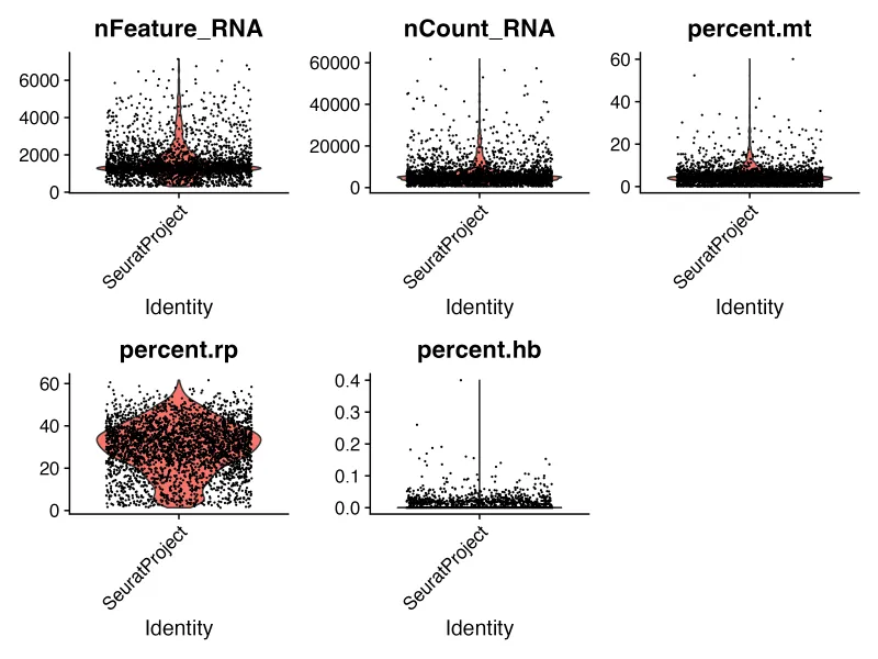
# VlnPlot观察各个指标情况
VlnPlot(sce, 
        features = c("nFeature_RNA",
                     "nCount_RNA", 
                     "percent.mt",
                     "percent.rp",
                     "percent.hb"), 
  ncol = 3,pt.size = 0.1, group.by = "orig.ident")
ggsave("VlnPlot.png",width = 8,height = 6,dpi = 300)

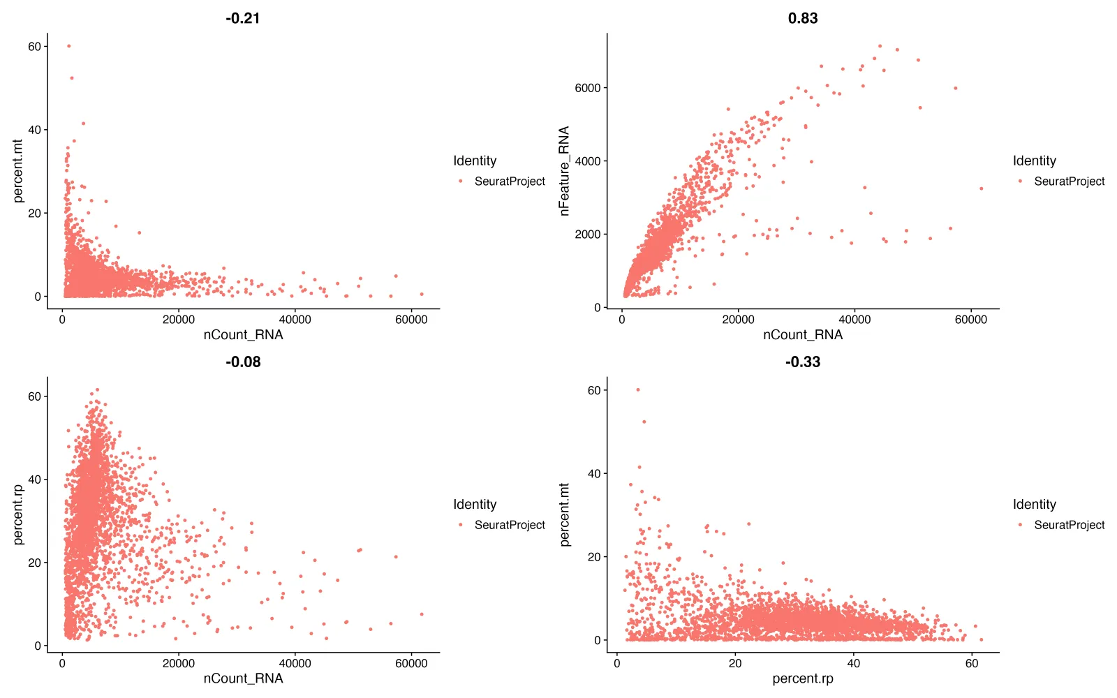
# 散点图-----Count_RNA和线粒体
plot1 <- FeatureScatter(sce, feature1 = "nCount_RNA", 
                        feature2 = "percent.mt",
                        group.by = "orig.ident")
#散点图-----Count_RNA和细胞数？
plot2 <- FeatureScatter(sce, feature1 = "nCount_RNA", 
                        feature2 = "nFeature_RNA",
                        group.by = "orig.ident")
# 散点图-----Count_RNA和核糖体
plot3 <- FeatureScatter(sce, feature1 = "nCount_RNA", 
                        feature2 = "percent.rp",
                        group.by = "orig.ident")
# 散点图-----核糖体和线粒体
plot4 <- FeatureScatter(sce, feature1 = "percent.rp", 
                        feature2 = "percent.mt",
                        group.by = "orig.ident")
plot1 + plot2 + plot3 + plot4
ggsave("FeatureScatter.png",width = 16,height = 10,dpi = 300)

# 根据图的结果进行细胞过滤，参数需要自行修改！！ 我这里的示例数据
seu.obj = subset(sce,
                nFeature_RNA < 6000 & 
                nCount_RNA < 30000 &
                percent.mt < 18 &
                percent.rp <15 &
                percent.hb <1)

nFeature_RNA：代表每个细胞中检测到的基因数量。
nCount_RNA：代表每个细胞中 RNA 分子的总数。高值可能表示高表达的细胞，但过高也可能是细胞双重性（doublets）或低质量细胞的标志。
percent.mt：代表每个细胞中线粒体基因的表达百分比。一般认为线粒体含量增高的细胞为裂解的细胞（死细胞），而活细胞中检测到的线粒体含量应低于10%。但如果是高代谢的细胞就需要谨慎过滤该指标。
percent.rp：代表每个细胞中核糖体蛋白基因的表达百分比。
percent.hb：代表血红蛋白基因的表达百分比。一般不研究这个可以过滤

主要查看左上角和右上角的两张图

1、左上角 (percent.mt vs. nCount_RNA)：相关性系数 (-0.21)：表现出负相关，这意味着 RNA 总数越多，线粒体基因的表达比例越低。这通常是期望的，因为高线粒体比例通常与细胞状态差（如细胞死亡）相关。

2、右上角 (nFeature_RNA vs. nCount_RNA)：相关性系数 (0.83)：表现出强正相关，说明随着 RNA 数量的增加，检测到的基因数目也在增加，这是预期的结果。

4、常规流程—数据标准化及高变基因

# 标准化数据
sce <- NormalizeData(sce, 
                     normalization.method = "LogNormalize", 
                     scale.factor = 10000)

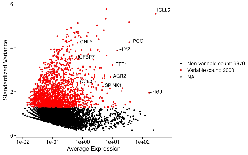
# 鉴定2000个高变基因(数量可人为设置，一般是2K)
sce <- FindVariableFeatures(sce, 
                            selection.method = "vst", 
                            nfeatures = 2000)
# 找出10个高变的基因
top10 <- head(VariableFeatures(sce), 10)

# 对高可变基因进行可视化
plot1 <- VariableFeaturePlot(sce)
plot2 <- LabelPoints(plot = plot1, points = top10, 
                     repel = TRUE);plot2
ggsave("Variablegenes.png",plot = plot2, width = 8,height = 5,dpi = 300)

4.1、常规流程-缩放数据

# 缩放数据保证每个基因在同一个尺度上
# 这个ScaleData 函数的 Default is variable features. 
# 如果我们不添加  features = all.genes ，
# 它就是默认的前面的 FindVariableFeatures 函数的2000个基因
all.genes <- rownames(sce)
sce <- ScaleData(sce, features = all.genes)

4.2、常规流程-PCA降维和harmony整合

除harmony之外有其他多种整合数据的方式

# PCA降维
sce <- RunPCA(sce,features = VariableFeatures(object = sce) , 
              #npcs = 20, # npcs = 20 表示计算并保留前20个主成分
              verbose = FALSE)
# sce@reductions$pca@cell.embeddings[1:4,1:4]
# 展示1和2主成分中的主要“荷载”
# VizDimLoadings(sce, dims = 1:2, reduction = "pca")
# Dimplot可视化
# DimPlot(sce, reduction = "pca",group.by = "orig.ident")
# heatmap可视化(可自行修改dims)
# DimHeatmap(sce, dims = 1, cells = 500, balanced = TRUE)


# 多种整合数据的方式
# CCA integration (method=CCAIntegration)
# RPCA integration (method=RPCAIntegration)
# Harmony (method=HarmonyIntegration)
# JointPCA (method= JointPCAIntegration)
# FastMNN (method= FastMNNIntegration)
# scVI (method=scVIIntegration)

# harmony整合
RunHarmony(sce,group.by.vars ="orig.ident")
# 如果seraut对象中没有保存harmony，那需要手动存储Harmony结果
# harmony_embeddings <- Embeddings(RunHarmony(sce,
                                            group.by.vars = "orig.ident"))
# sce[["harmony"]] <- CreateDimReducObject(embeddings = harmony_embeddings,
                                         key = "harmony_",
                                         assay = DefaultAssay(sce))

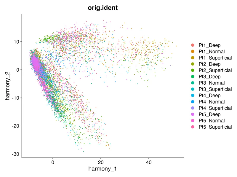
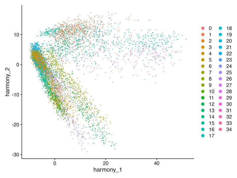
#harmony降维后的可视化
DimPlot(sce, reduction = "harmony", group.by = "orig.ident")
ggsave("harmony_orig.png",width = 8,height = 6,dpi = 300)
sce <- JoinLayers(sce)

#单样本的时候需要通过下面的代码去选择pca降维后的数量
#接下来我们既然已经对庞大的数据进行了降维（也就是聚堆）的形式，那么我们究竟要选择几个PC来代表这么庞大的数据呢，肯定不能都选，否则我的数据量还是这些，就没有我们前面一直渗透的缩小缩小再缩小的含义了
# sce <- JackStraw(sce, num.replicate = 100)
# sce <- ScoreJackStraw(sce, dims = 1:20) #dims最大是20
# #上面两个代码是通过不同的方式来帮助我们选择PC的数目，并且分别都对应不同的可视化
# JackStrawPlot(sce, dims = 1:20) #最大值是20

#harmony函数只能用ElbowPlot去分析
ElbowPlot(sce,ndims=50)
ggsave("ElbowPlot.png",width = 8,height = 6,dpi = 300)
#不同的判断方法选择的PC数是不一样的，而且理论上来说保存更多的PC可以保存更多的生物学差异，所以这里我们灵活选择即可，因为都不算错

从下面的图中需要挑选一个合适的ndims值

4.3、cluster分群-harmony可视化

# 基于降维后的数据构建细胞邻近图
# dims的数量是根据上一步所确定的ElbowPlot
dims_N <- "30" 
sce <- FindNeighbors(sce, dims = 1:dims_N, 
                     reduction = "harmony", #单样本需要pca
                     verbose = FALSE) 

# 进行聚类分析，基于邻近图(之前由FindNeighbors 函数构建)划分细胞群体
# 可以通过Idents(sce) 对比前后的levels数量变化
# 请注意，我这边resolution设置了一个梯度
sce <- FindClusters(sce, 
                    resolution = seq(0.1, 2, by = 0.1), 
                    verbose = FALSE)
head(Idents(sce), 5)

#可视化cluster
cluster_harmony <- DimPlot(sce, reduction = "harmony");print(cluster_harmony) #单样本需要pca
ggsave("cluster_harmony.png",plot = cluster_harmony,
       width = 8,height = 6,dpi = 300)

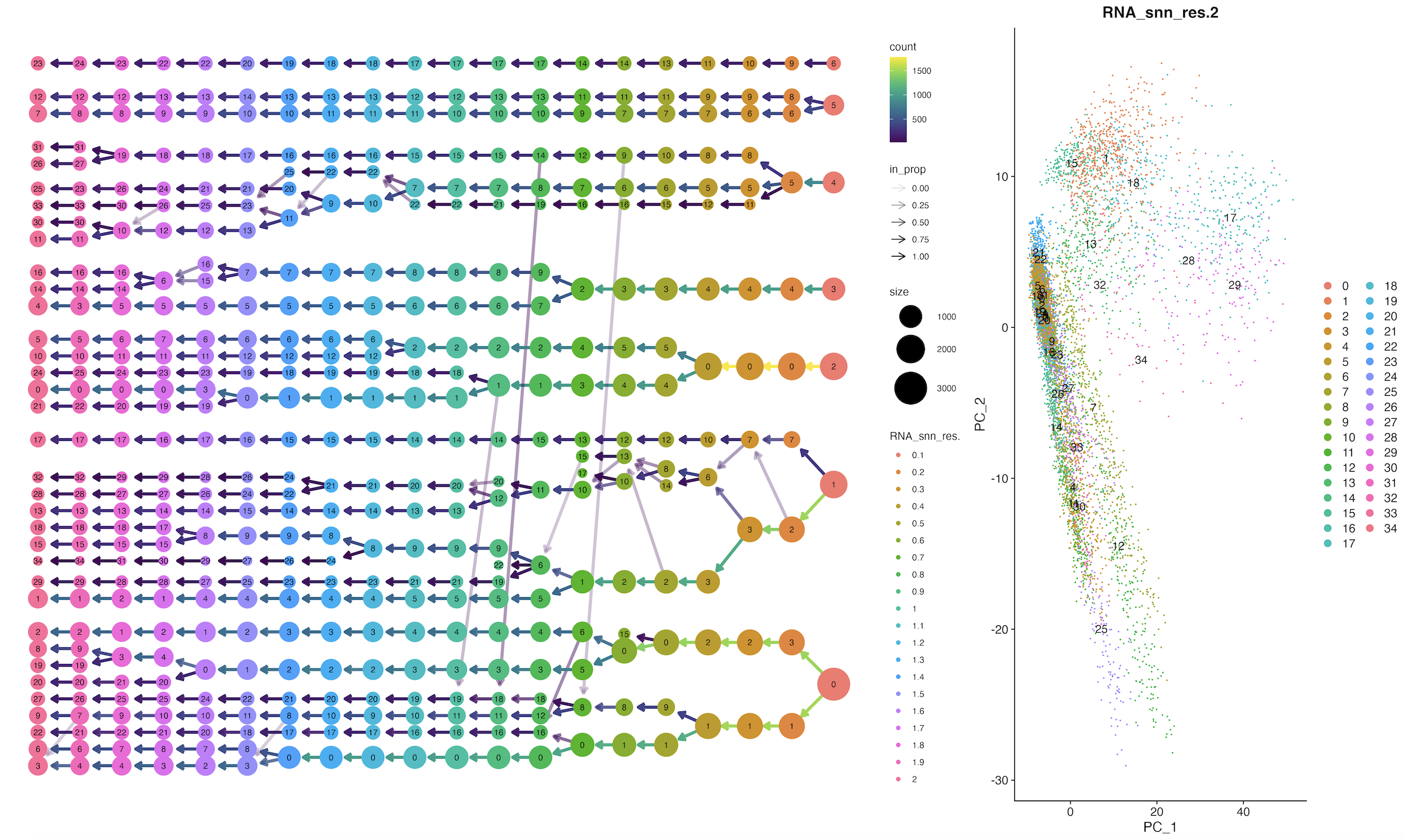
4.4、clustree图

library(clustree)
library(patchwork)
p1 <- clustree(sce, prefix = 'RNA_snn_res.') + coord_flip();p1
#这里的RNA_snn_res后面的数值是可以修改的
p2 <- DimPlot(sce, group.by = 'RNA_snn_res.2', label = T);p2 
Tree_1 <- p1 + p2 + plot_layout(widths = c(3, 1));print(Tree_1)
ggsave("cluster_tree.png",plot = Tree_1, 
       width = 20,height = 12,dpi = 300)

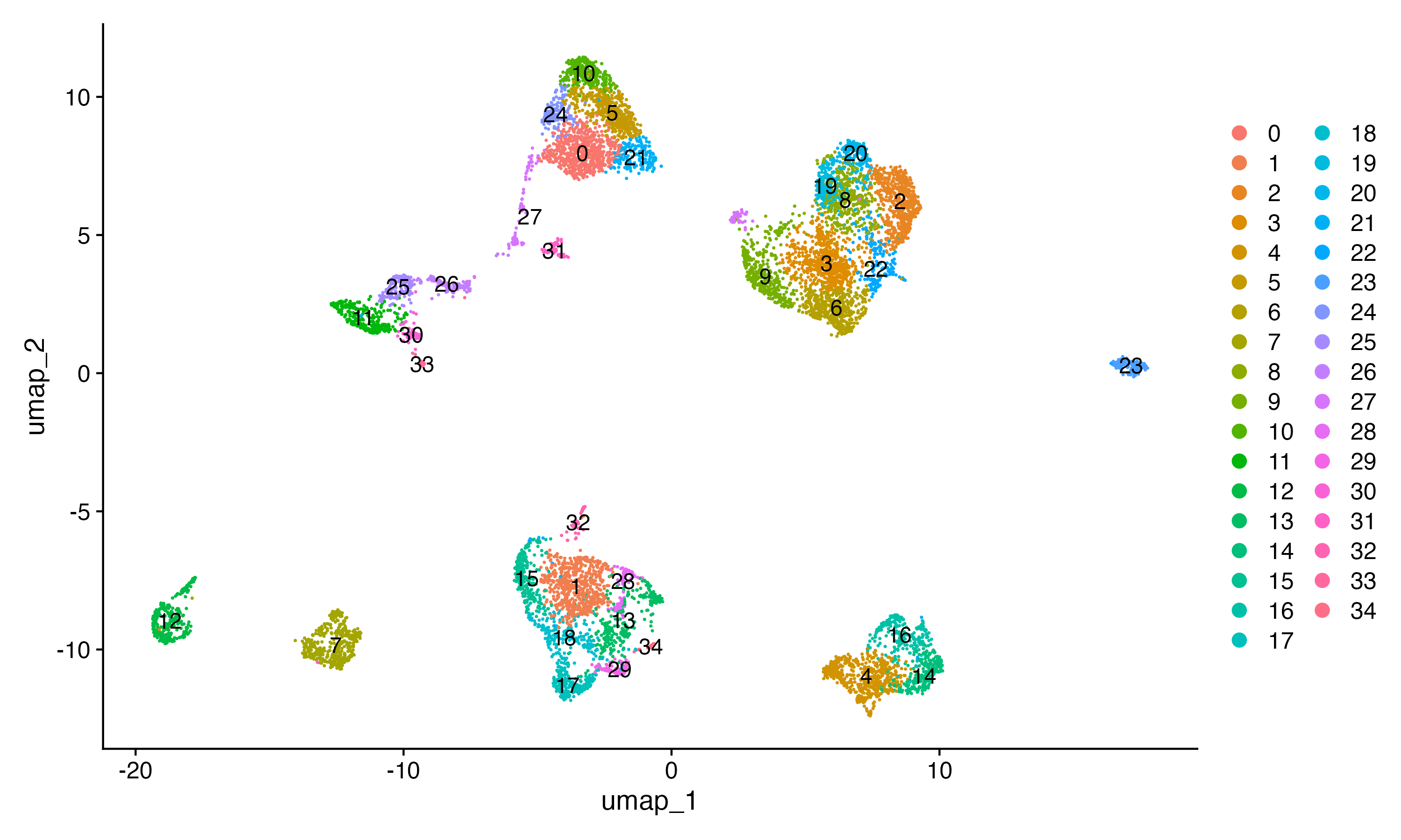
4.5、UMAP/tSNE可视化

#UMAP/tSNE可视化前先确定一个想要的reslution值
#这里重新跑一遍之后后面就会按照新跑的reslution值进行分析
sce <- FindClusters(sce, resolution = 2, verbose = FALSE)

#假设电脑的显卡非常高级的话，可以不用PCA降维，直接UMAP
#Umap方式
sce <- RunUMAP(sce, dims = 1:dims_N, 
               umap.method = "uwot", metric = "cosine")
sce <- JoinLayers(sce)
UMAP_1 <- DimPlot(sce,label = T);print(UMAP_1)
ggsave("UMAP.png",plot = UMAP_1,width = 10,height = 6,dpi = 300)
#Tsne方式
#pbmc <- RunTSNE(pbmc )
#DimPlot(pbmc,label = T,reduction = 'tsne',pt.size =1)

5、细胞亚群注释前marker提取

#首先要确认一下每一cluster中的marker基因
#其中pct.1：在目标细胞簇中表达的细胞比例;pct.2：在其他细胞簇中表达的细胞比例。
sce.markers <- FindAllMarkers(sce, only.pos = TRUE, 
                              min.pct = 0.25, 
                              logfc.threshold = 0.25, 
                              verbose = FALSE)
head(sce.markers,n = 5)
write.csv(sce.markers, "sce_all_markers.csv", row.names = TRUE)

#显示每个簇中log2FC表达最高5个值
a <- sce.markers %>%
   group_by(cluster) %>% # dplyr包中的函数可以进行分组操作
   top_n(n = 5, wt = avg_log2FC)%>% # dplyr包中的函数，可以提取前多少行
   data.frame()
write.csv(a, "sce_markers_top5.csv", row.names = TRUE)


#可视化
seurat_cluster <- DimPlot(sce, reduction = "umap", 
                          group.by = 'seurat_clusters',
                          label = TRUE, pt.size = 0.5);print(seurat_cluster)
ggsave("seurat_cluster.png",plot = seurat_cluster, 
       width = 10,height = 6,dpi = 300)

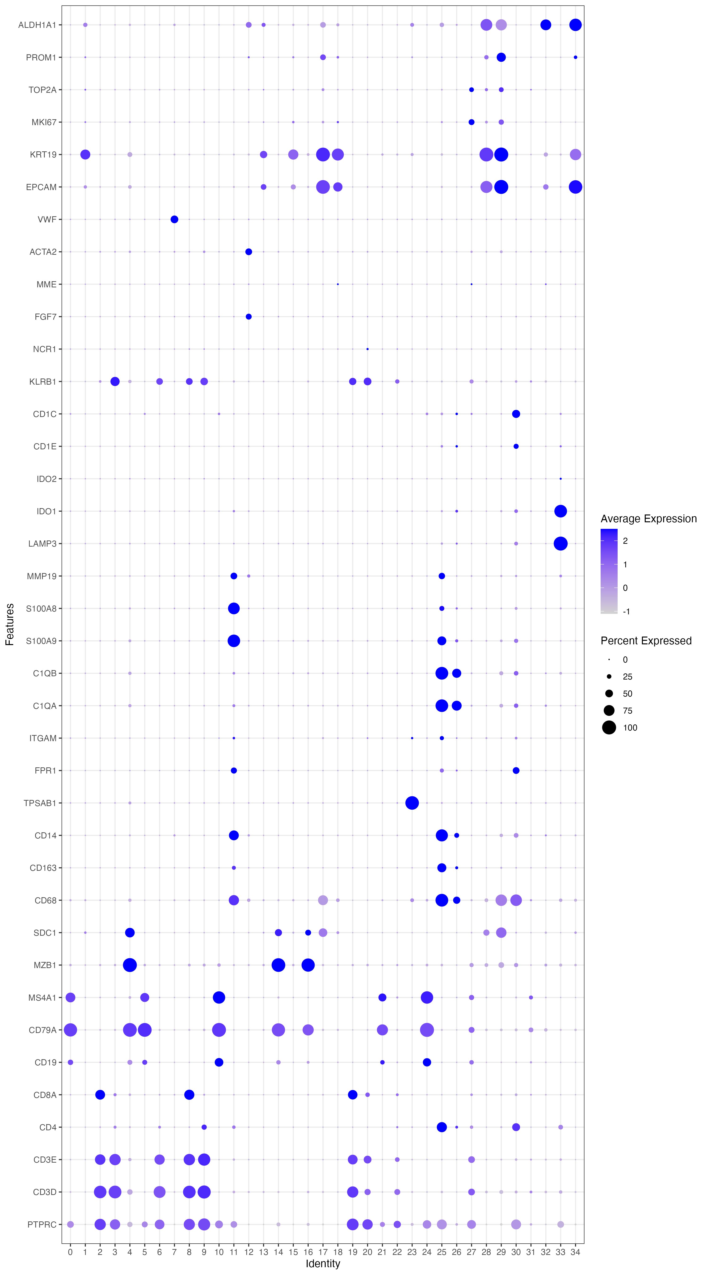
#所有的marker进行绘图
sce_all = sce
library(ggplot2) 
genes_to_check = c('PTPRC', 'CD3D', 'CD3E', 'CD4','CD8A',
                   'CD19', 'CD79A', 'MS4A1' ,
                   'IGHG1', 'MZB1', 'SDC1',
                   'CD68', 'CD163', 'CD14', 
                   'TPSAB1' , 'TPSB2',  # mast cells,
                   'RCVRN','FPR1' , 'ITGAM' ,
                   'C1QA',  'C1QB',  # mac
                   'S100A9', 'S100A8', 'MMP19',
                   'LAMP3', 'IDO1','IDO2', 
                   'CD1E','CD1C', # DC2
                   'KLRB1','NCR1', # NK 
                   'FGF7','MME', 'ACTA2', 
                   'PECAM1', 'VWF',  
                   'EPCAM', 'KRT19',
                   'MKI67','TOP2A', 
                   'PROM1', 'ALDH1A1' )
library(stringr)   
p_all_markers <- DotPlot(sce_all , 
                         features = genes_to_check,
                         assay='RNA',
                         group.by = 'seurat_clusters')  + 
                 coord_flip() + 
                 theme_bw()  # 添加其他主题或元素
p_all_markers 
ggsave('p_all_markers.pdf',width = 10,height = 8)

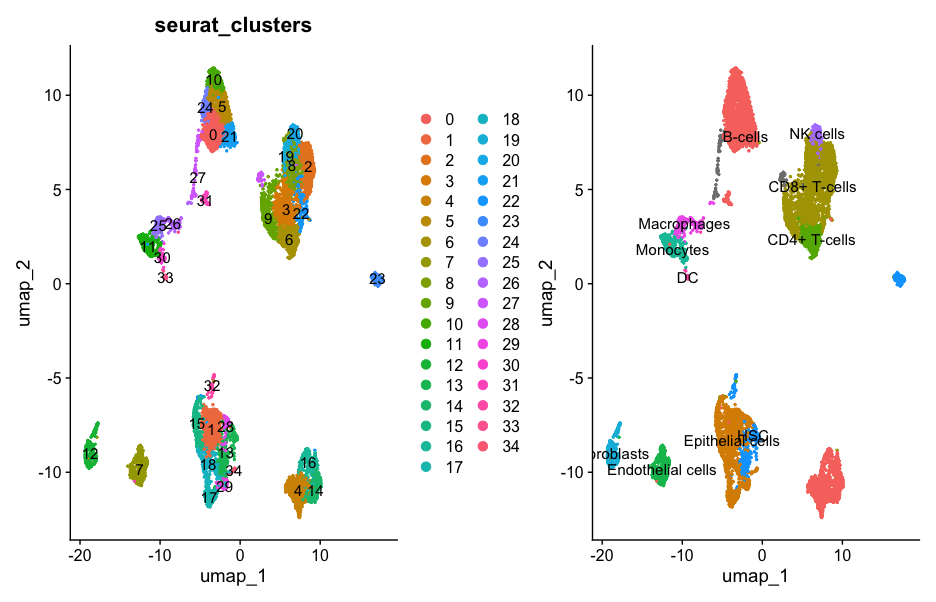
6.cluster合并

本次采用SingleR注释

library(celldex)
ls("package:celldex")
BlueprintEncode <- BlueprintEncodeData()

library(SingleR)
library(BiocParallel)
scRNA = sce
# 提取归一化数据
test <- GetAssayData(scRNA, layer = "data")
table(scRNA@active.ident)
Rename_scRNA <- SingleR(test = test, 
                        ref = BlueprintEncode, # 参考注释文件
                        labels = BlueprintEncode$label.main,  #标注信息
                        clusters = scRNA@active.ident)

Rename_scRNA$pruned.labels
#  [1] "B-cells"           "Epithelial cells"  "CD8+ T-cells"      "CD8+ T-cells"      "B-cells"          
#  [6] "B-cells"           "CD4+ T-cells"      "Endothelial cells" "CD8+ T-cells"      "CD8+ T-cells"     
# [11] "B-cells"           "Monocytes"         "Fibroblasts"       "HSC"               "B-cells"          
# [16] "Epithelial cells"  "B-cells"           "Epithelial cells"  "Epithelial cells"  "CD8+ T-cells"     
# [21] "NK cells"          "B-cells"           "CD8+ T-cells"      "HSC"               "B-cells"          
# [26] "Macrophages"       "Macrophages"       NA                  "Epithelial cells"  "Epithelial cells" 
# [31] "Monocytes"         "B-cells"           "HSC"               "DC"                "Epithelial cells" 

new.cluster.ids <- Rename_scRNA$pruned.labels
names(new.cluster.ids) <- levels(scRNA)
scRNA <- RenameIdents(scRNA,new.cluster.ids)
p2 <- DimPlot(scRNA, reduction = "umap",label = T,pt.size = 0.5) + NoLegend()
seurat_cluster+p2

人工注释-这里是示例！！需要自行修改

# 命名是完全依赖生物学背景！先定义一个new.cluster.ids
# 这里的群的命名需要自行
#####细胞生物学命名
celltype=data.frame(ClusterID=0:24,
                    celltype= 0:24) 

# 这里强烈依赖于生物学背景，看dotplot的基因表达量情况来人工审查单细胞亚群名字
celltype[celltype$ClusterID %in% c(3,5,11,13,14,21 ),2]='epithelial'
celltype[celltype$ClusterID %in% c(12,23 ),2]='myeloid'
celltype[celltype$ClusterID %in% c(2,8,10,17,18,22 ),2]='B'
celltype[celltype$ClusterID %in% c(0,1,4,6,7,9,16,24 ),2]='T'
celltype[celltype$ClusterID %in% c(15,20 ),2]='fibroblasts'
celltype[celltype$ClusterID %in% c(19 ),2]='endothelial'

table(scRNA@meta.data$RNA_snn_res.1)
table(celltype$celltype)

# 这里的RNA_snn_res需要自行修改！
scRNA@meta.data$celltype = "NA"
for(i in 1:nrow(celltype)){
  scRNA@meta.data[which(scRNA@meta.data$RNA_snn_res.2 == celltype$ClusterID[i]),'celltype'] <- celltype$celltype[i]}
table(scRNA@meta.data$celltype)

#这里把levels赋值到new.cluster.ids上去
names(new.cluster.ids) <- levels(scRNA)
# 修改Idents中分群编号为细胞类型
scRNA <- RenameIdents(scRNA, new.cluster.ids)
y <- DimPlot(scRNA, reduction = "umap", label = TRUE,  
             repel = T,pt.size = 0.5) + 
             NoLegend() #这个是隐藏图注
print(y)
ggsave('cluster_new.png',plot = y, 
       width = 10,height = 8,dpi = 300)

致谢：感谢曾老师以及生信技能树团队全体成员。

注：若对内容有疑惑或者有发现明确错误的朋友，请联系后台(欢迎交流)。更多内容可关注公众号：生信方舟

- END -