文章MSM_metagenomics（六）：复杂热图绘制

欢迎大家关注全网生信学习者系列：

• WX公zhong号：生信学习者
• Xiao hong书：生信学习者
• 知hu：生信学习者
• CDSN：生信学习者2

介绍

本教程将使用基于R的函数在复杂热图上绘制物种的丰度或流行度。

数据

大家通过以下链接下载数据：

• 百度网盘链接：https://pan.baidu.com/s/1f1SyyvRfpNVO3sLYEblz1A
• 提取码: 请关注WX公zhong号_生信学习者_后台发送 复现msm 获取提取码

R packages required

• ComplexHeatmap

• grid

R packages optional

• viridis

• circlize

Visualize species relative abundances (or presence/absence) by plotting ComplexHeatmap

使用complexheatmap_plotting_funcs.R 画图。

complexheatmap_plotting_funcs.R函数参考R可视化：微生物相对丰度或富集热图可视化

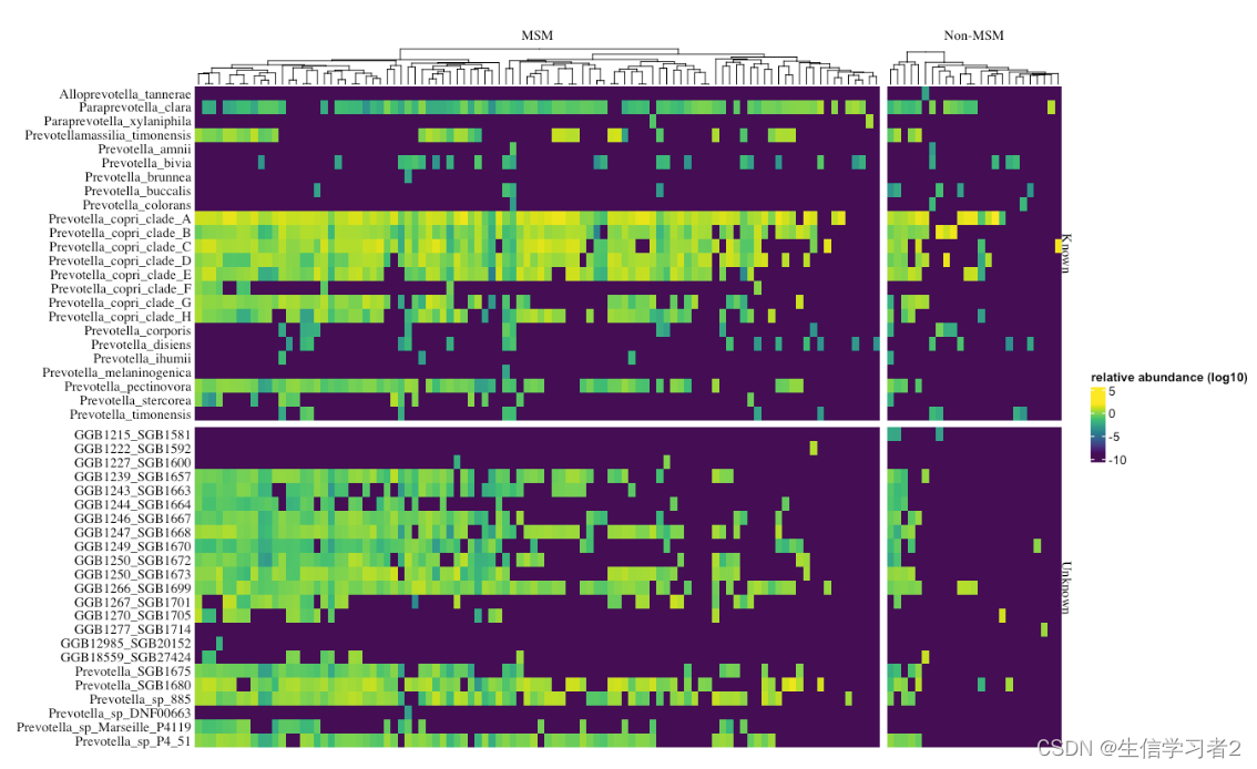
示例1: Visualize Prevotellaceae community

指定一个由MetaPhlAn量化的Prevotellaceae物种相对丰度的矩阵表matrix table。可选地，还可以提供一个与矩阵表matrix table逐行匹配的行分组文件row-grouping file，以及一个与矩阵表逐列匹配的列分组文件column-grouping file。

prevotellaceae_mat <- "./data/prevotellaceae_matrix_4ComplexHeatmap.tsv"
prevotellaceae_row_groups <- "./data/prevotellaceae_matrix_4ComplexHeatmap_species_md.txt"
prevotellaceae_col_groups <- "./data/prevotellaceae_matrix_4ComplexHeatmap_sample_md.txt"

一旦指定了输入文件，现在我们可以使用可视化函数plot_complex_heatmap，该函数实现了ComplexHeatmap 来绘制热图，并附加其他信息，通过指定参数：

• mat_file: the relative abundance file in metaphlan-style, [tsv file].
• column_md: the column-grouping file in which each row matches the column of mat_file, [txt file].
• row_md: the row-grouping file in which each row matches the row of mat_file, [txt file].
• color_bar_name: the title for color bar scale, [string], default: [NULL].
• transformation: the transformation function for values in mat_file, including log10([log10]), squared root arcsin ([sqrt_asin]) and binary([binary]), default: [NULL].
• font_style: the font style for all labels in the plot, [string], default: [“Arial”].
• font_size: the font size for all labels in the plot, [int], default: [11].
• show_col_names: display column names, [TRUE/FALSE], default: [TRUE].
• show_row_names: display row names, [TRUE/FALSE], default: [TRUE].
• row_names_side: specify the side you would like to place row names, [string], default: [left].
• column_names_side: specify the side you would like to place row names, [string], default: [bottom].
• cluster_columns: cluster columns where values are similar, [TRUE/FALSE], default: [FALSE].
• cluster_rows: cluster rows where values are similar, [TRUE/FALSE], default: [FALSE].
• cluster_row_slices: reorder row-wise slices (you can call them batches too) where values of slices are similar, [TRUE/FALSE], default: [FALSE].
• cluster_column_slices: reorder column-wise slices (you can call them batches too) where values of slices are similar, [TRUE/FALSE], default: [FALSE].
• color_func: define custom color function to show values, default: [NULL].
• border: add board to the plot, [TRUE/FALSE], default: [FALSE].
• row_gap: control gap distance between row slices if you used row_md argument, [float], default: [1].
• column_gap: control gap distance between column slices if you used column_md argument, [float], default: [1].
• width: control the width of the whole complex heatmap, [float], default: [1].
• height: control the height of the whole complex heatmap, [float], default: [1].

在这里，我们通过一个示例展示了在MSM和Non-MSM个体中Prevotellaceae群落的相对丰度的可视化。

col_func <- viridis::viridis(100) # define the color palette using viridis function.

plot_complex_heatmap(
  prevotellaceae_mat,
  color_bar_name = "relative abundance (log10)",
  row_md = prevotellaceae_row_groups,
  column_md = prevotellaceae_col_groups,
  show_col_names = FALSE,
  show_row_names = TRUE,
  width = 2,
  height = 4,
  row_names_side = "left",
  cluster_columns = TRUE,
  cluster_column_slices = FALSE,
  cluster_rows = FALSE,
  cluster_row_slices = FALSE,
  border = FALSE,
  row_gap = 2,
  column_gap = 2,
  color_func = col_func,
  transformation = "log10")

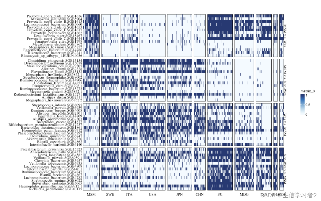
示例2: Visualize presence and absence of a group of species across global populations

现在，我们将使用相同的策略来可视化全球人群中在存在和缺失方面重要的一系列物种。分类学矩阵文件 taxonomic matrix file包含了60种在MSM、西方化或非西方化个体中发现富集的物种，它们的组别可以在行分组文件row-group file中找到。此外，分类学矩阵文件taxonomic matrix file中的大约1000个样本来自MSM和10个国家，它们的组别可以在列分组文件column-grouping file中找到。

global_mat <- "./data/global_enrichment_matrix.tsv"
global_row_md <- "./data/global_enrichment_matrix_rownames.tsv"
global_col_md <- "./data/global_enrichment_matrix_colnames.tsv"

col_func <- circlize::colorRamp2(c(0, 1), hcl_palette = "Blues", reverse = T)

plot_complex_heatmap(
  global_mat,
  row_md = global_row_md,
  column_md = global_col_md,
  show_col_names = F,
  show_row_names = TRUE,
  width = 0.2,
  height = 3,
  row_names_side = "left",
  column_names_side = "top",
  cluster_columns = F,
  cluster_column_slices = F,
  cluster_rows = F,
  cluster_row_slices = F,
  border = T,
  row_gap = 2,
  column_gap = 2,
  color_func = col_func2,
  transformation = "binary")