文章MSM_metagenomics（八）：机器学习分析

最新推荐文章于 2024-06-27 22:35:56 发布

生信学习者2

最新推荐文章于 2024-06-27 22:35:56 发布

阅读量1k

点赞数 27

分类专栏：复现文章文章标签：机器学习数据分析

本文链接：https://blog.csdn.net/H20230717/article/details/139765465

版权

复现文章专栏收录该内容

18 篇文章 0 订阅

订阅专栏

欢迎大家关注全网生信学习者系列：

WX公zhong号：生信学习者
Xiao hong书：生信学习者
知hu：生信学习者
CDSN：生信学习者2

介绍

本教程是使用随机森林模型来评估微生物群落分类组成预测能力。

数据

大家通过以下链接下载数据：

百度网盘链接：https://pan.baidu.com/s/1f1SyyvRfpNVO3sLYEblz1A
提取码: 请关注WX公zhong号_生信学习者_后台发送 复现msm 获取提取码

Evaluate the predictive power of microbiome taxonomic composition

Python package required

Random forest training and results evaluation with ROC-AUC curve

在这里，我们将介绍一个Python脚本evaluation_kfold.py，该脚本实现了random forest model模型，用于评估微生物群落分类组成中编码的信息对不同个体分类的预测能力

代码

#!/usr/bin/env python

"""
NAME: evaluation_kfold.py
DESCRIPTION: This script is to evaluate a model's prediction power using tenfold method.
"""

from sklearn.model_selection import train_test_split
from sklearn.ensemble import RandomForestClassifier
from sklearn import metrics
from collections import namedtuple
from sklearn.calibration import CalibratedClassifierCV
from sklearn.feature_selection import SelectFromModel
import pandas as pd
import itertools 
import sys
import argparse
import textwrap
import subprocess
import random
import numpy as np
from sklearn.model_selection import StratifiedKFold
from sklearn.metrics import roc_curve
from sklearn.metrics import roc_auc_score
import matplotlib.pyplot as plt
from sklearn.metrics import auc
from sklearn.metrics import RocCurveDisplay
import matplotlib

matplotlib.rcParams['font.family'] = 'sans-serif'
matplotlib.rcParams['font.sans-serif'] = 'Arial'

def read_args(args):
    # This function is to parse arguments

    parser = argparse.ArgumentParser(formatter_class=argparse.RawDescriptionHelpFormatter,
                                    description = textwrap.dedent('''\
                                    This script is to estimate ROC AUC based on metaphlan-style table with metadata being inserted.
                                    '''),
                                    epilog = textwrap.dedent('''\
                                    examples: evaluation_kfold.py --mpa_df <mpa_df.tsv> --md_rows 0,1,2,3,4 --target_row 3 --pos_feature <CRC> --neg_feature <Healthy> --fold_number 10 --repeat_time 20 --output ROC_AUC.svg  
                                    '''))

    parser.add_argument('--mpa_df',
                        nargs = '?',
                        help = 'Input a mpa-style table with metadata being inserted.',
                        type = str,
                        default = None)

    parser.add_argument('--md_rows',
                        nargs = '?',
                        help = 'Input row numbers for specifying metadata without considering header row, zero-based, comma delimited. for example, 0,1,2,3,4.',
                        default = None)

    parser.add_argument('--target_row',
                        nargs = '?',
                        help = 'Specify the row number for indicating target metadata to examine, zero-based without considering header row.',
                        type = int,
                        default = None)

    parser.add_argument('--pos_feature',
                        nargs = '?',
                        help = 'Specify the feature name to be labeled as posive, e.g. 1.',
                        type = str,
                        default = None)

    parser.add_argument('--neg_feature',
                        nargs = '?',
                        help = 'Specify the feature name to be labeld as negative, e.g. 0.',
                        type = str,
                        default = None)

    parser.add_argument('--fold_number',
                        nargs = '?',
                        help = 'Specify the fold number you want split the whole dataset.',
                        type = int,
                        default = None)

    parser.add_argument('--repeat_time',
                        nargs = '?',
                        help = 'Specify the repeat time you want to split the dataset.',
                        type = int,
                        default = None)

    parser.add_argument('--output',
                        nargs = '?',
                        help = 'Specify the output figure name.',
                        type = str,
                        default = None)

    parser.add_argument('--output_values',
                        nargs = '?',
                        help = 'Specify the output file name for storing ROC-AUC values.',
                        type = str,
                        default = None)

    parser.add_argument('--nproc',
                        nargs = '?',
                        help = 'Specify the number of processors you want to use. 4 by default.',
                        type = int,
                        default = 4)

    parser.add_argument('--transform',
                        nargs = '?',
                        help = 'Transform values in the matrix, [arcsin_sqrt] or [binary] or [None]. [None] by default',
                        type = str,
                        default = None)

    return vars(parser.parse_args())



def get_df_dropping_metadata(mpa4_df, row_number_list):
    # row_number_list: a list of row numbers in integer.
    # this function is to drop rows containing metadata.

    df_ = df_.drop(row_number_list)

    return df_

def get_target_metadata(mpa4_df, row_number):
    # row_number: the integer indicating the row which contains the metadata one wants to examine.
    # this function is to get a list of binary metadata for establishing ML model.
    
    features = mpa4_df.iloc[row_number].to_list()

    return features

def prepare_dataset(mpa4_style_md_df, pos_neg_dict, row_number_list, target_row, transform):
    # mpa4_style_md_df: the merged metaphlan4 table with metadata being inseted.
    # pos_neg_dict: the dictionary which maps examine value to 1 or 0.
    # This function is to prepare dataset for downstream analysis.

    df_no_md = mpa4_style_md_df.drop(row_number_list)
    sample_names = df_no_md.columns[1:].to_list()
    matrix = []
    for s in sample_names:
        values = [float(i) for i in df_no_md[s].to_list()]
        matrix.append(values)

    matrix = np.array(matrix)
    
    if transform == 'arcsin_sqrt':
        matrix = matrix/100
        print(matrix)
        matrix = np.arcsin(np.sqrt(matrix))

    elif transform == 'binary':
        matrix[np.where(matrix > 0)] = 1
    else:
        matrix = matrix

    features = get_target_metadata(mpa4_style_md_df, target_row)[1:]

    X = np.asarray(matrix)
    y = [pos_neg_dict[i] for i in features]
    y = np.asarray(y)

    return X, y


def roc_auc_curve(model, X, y, fold, repeat, output_name, output_values):
    # model: machine learning model to use.
    # X: the value matrix
    # y: the list of features, 1 and 0
    # fold: the number of fold to split the dataset.
    # repeat: the repeat number for splitting the dataset.
    # output_name: specify the output figure name.
    # outout_values: specify the output file name for storing estimated roc-auc values.

    cv = StratifiedKFold(n_splits=fold, shuffle=True)
    classifier = model

    tprs = []
    aucs = []
    mean_fpr = np.linspace(0, 1, 100)
    
    rocauc_opt = open(output_values, "w")

    rocauc_opt.write("repeat"+ "\t" + "fold" + "\t" + "roc_auc" + "\n")
    while repeat > 0:
        repeat -= 1
        for i, (train, test) in enumerate(cv.split(X, y)):
            classifier.fit(X[train], y[train])
            viz = RocCurveDisplay.from_estimator(
                classifier,
                X[test],
                y[test],
                name="ROC fold {}".format(i),
                alpha=0.3,
                lw=1,
            )
            interp_tpr = np.interp(mean_fpr, viz.fpr, viz.tpr)
            interp_tpr[0] = 0.0
            tprs.append(interp_tpr)
            aucs.append(viz.roc_auc)
            rocauc_opt.write(str(repeat) + "\t" + str(i) + "\t" + str(viz.roc_auc) + "\n")

    fig, ax = plt.subplots()
    ax.plot([0, 1], [0, 1], linestyle="--", lw=2, color="r", label="Chance", alpha=0.8)
    mean_tpr = np.mean(tprs, axis=0)
    mean_tpr[-1] = 1.0
    mean_auc = auc(mean_fpr, mean_tpr)
    std_auc = np.std(aucs)
    ax.plot(
        mean_fpr,
        mean_tpr,
        color="b",
        label=r"Mean ROC (AUC = %0.2f $\pm$ %0.2f)" % (mean_auc, std_auc),
        lw=2,
        alpha=0.8,
    )
    std_tpr = np.std(tprs, axis=0)
    tprs_upper = np.minimum(mean_tpr + std_tpr, 1)
    tprs_lower = np.maximum(mean_tpr - std_tpr, 0)
    ax.fill_between(
    mean_fpr,
    tprs_lower,
    tprs_upper,
    color="grey",
    alpha=0.2,
    label=r"$\pm$ 1 std. dev.",
    )
    ax.set(
        xlim=[-0.05, 1.05],
        ylim=[-0.05, 1.05],
    )
    ax.set_xlabel('False Positive Rate')
    ax.set_ylabel('True Positive Rate')
    ax.legend(loc="lower right")
    plt.savefig(output_name)
    rocauc_opt.close()



if __name__ == "__main__":

    pars = read_args(sys.argv)
    df = pd.read_csv(pars["mpa_df"], sep = "\t", index_col = False)
    row_number_list = [int(i) for i in pars["md_rows"].split(",")]
    pos_neg_dict = {pars["pos_feature"]:1, pars["neg_feature"]:0}
    X, y = prepare_dataset(df, pos_neg_dict, row_number_list, pars["target_row"], pars["transform"])
    model = RandomForestClassifier(n_estimators = 1000,
                                   criterion = 'entropy',
                                   min_samples_leaf = 1,
                                   max_features = 'sqrt',
                                   n_jobs = 4) # initiating a RF classifier
    roc_auc_curve(model, X, y, pars["fold_number"], pars["repeat_time"], pars["output"], pars["output_values"])

用法

evaluation_kfold.py [-h] [--mpa_df [MPA_DF]] [--md_rows [MD_ROWS]] [--target_row [TARGET_ROW]] [--pos_feature [POS_FEATURE]] [--neg_feature [NEG_FEATURE]] [--fold_number [FOLD_NUMBER]] [--repeat_time [REPEAT_TIME]] [--output [OUTPUT]]
                           [--output_values [OUTPUT_VALUES]] [--nproc [NPROC]] [--transform [TRANSFORM]]

This script is to estimate ROC AUC based on metaphlan-style table with metadata being inserted.

optional arguments:
  -h, --help            show this help message and exit
  --mpa_df [MPA_DF]     Input a mpa-style table with metadata being inserted.
  --md_rows [MD_ROWS]   Input row numbers for specifying metadata without considering header row, zero-based, comma delimited. for example, 0,1,2,3,4.
  --target_row [TARGET_ROW]
                        Specify the row number for indicating target metadata to examine, zero-based without considering header row.
  --pos_feature [POS_FEATURE]
                        Specify the feature name to be labeled as posive, e.g. 1.
  --neg_feature [NEG_FEATURE]
                        Specify the feature name to be labeld as negative, e.g. 0.
  --fold_number [FOLD_NUMBER]
                        Specify the fold number you want split the whole dataset.
  --repeat_time [REPEAT_TIME]
                        Specify the repeat time you want to split the dataset.
  --output [OUTPUT]     Specify the output figure name.
  --output_values [OUTPUT_VALUES]
                        Specify the output file name for storing ROC-AUC values.
  --nproc [NPROC]       Specify the number of processors you want to use. 4 by default.
  --transform [TRANSFORM]
                        Transform values in the matrix, [arcsin_sqrt] or [binary] or [None]. [None] by default

examples: 

python evaluation_kfold.py --mpa_df <mpa_df.tsv> --md_rows 0,1,2,3,4 --target_row 3 --pos_feature <CRC> --neg_feature <Healthy> --fold_number 10 --repeat_time 20 --output ROC_AUC.svg

为了演示这个教程，我们使用了一个微生物组数据集machine_learning_input.tsv: ./data/machine_learning_input.tsv，其中包含52名受试者（28名受试者有超过3个性伴侣，24名受试者有0-3个性伴侣）以及相应的肠道微生物群落物种的相对丰度。

示例命令:

python evaluation_kfold.py \
  --mpa_df machine_learning_input.tsv \
  --md_rows 0 \
  --target_row 0 \
  --pos_feature ">3" \
  --neg_feature "0_3" \
  --fold_number 3 \
  --repeat_time 50 \
  --output roc_auc_npartners.png \
  --output_values roc_auc_npartners_values.tsv \
  --nproc 10

它生成了一个ROC-AUC曲线，以展示随机森林模型拟合我们输入的微生物群落分类数据的整体预测能力。

在这里插入图片描述

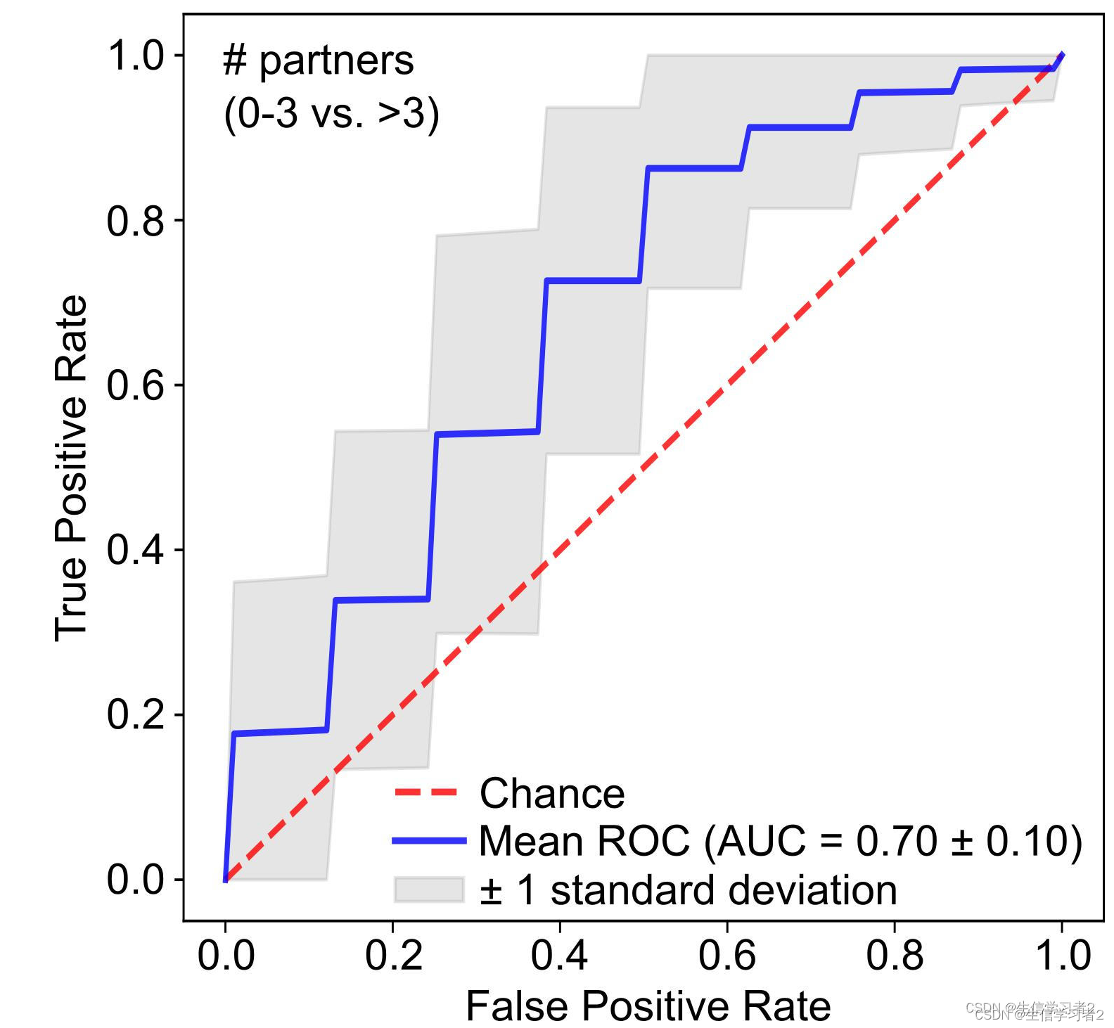
可选地，它还可以生成用于生成上述图表的原始输出roc_auc_npartners_values.tsv: ./data/roc_auc_npartners_values.tsv。人们可以将其用于其他目的。

Visualize standard deviation of machine learning estimates

R packages required

Plot the distribution of ROC-AUC estimates with standard deviation

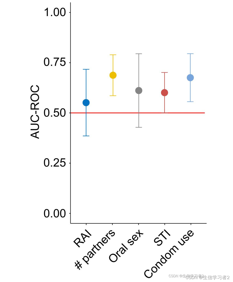
我们上面展示了如何使用ROC-AUC曲线通过与随机效应的基准测试来评估微生物群落的预测能力。在这里，我们将介绍在rocauc_stdv_funcs.R中实现的辅助函数data_summary和std_deviation_plot，用于可视化来自多次随机森林分类的结果的ROC-AUC估计的标准偏差。

data_summary is function to summarize raw ROC-AUC estimates in standard deviation with three arguments:

data: Input a dataframe as input.
var_estimates: The column header indicating ROC-AUC estimates for the target variable.
groups: The column header containing the group names.

std_deviation_plot is a function to plot ROC-AUC estimates with error bars based on standard deviation with arguments:

df: Input the dataframe of standard deviations of ROC-AUC estimates.
x_axis: Specify the column header (groups usually) for X axis.
y_axis: Specify the column header (ROC-AUC means usually) for Y axis.
stdv_column: Specify the column header indicating standard deviation.
palette: Specify the palette for colors, default [jco].
y_label: Name the Y label, default [ROC-AUC].
x_label: Name the X laebl, default NULL.
order_x_axis: give a vector to specify the order of columns along X axis.
font_size: specify the font size, default [11].
font_family: specify the font family, default [Arial].

在这里，我们将使用演示数据merged ROC-AUC estimates: ./data/roc_auc_merged.tsv合并的ROC-AUC估计值，这些数据来自于执行随机森林分类以区分五种性行为，包括接受receptive anal intercourse, number of partners, oral sex, sex transmitted infection, 和 condom use。

加载rocauc_stdv_funcs.R（包含data_summary和std_deviation_plot函数）。

data_summary <- function(data,
                         var_estimates,
                         groups){
  require(plyr)
  summary_func <- function(x, col){
    c(mean = mean(x[[col]], na.rm=TRUE),
      sd = sd(x[[col]], na.rm=TRUE))
  }
  data_sum<-ddply(data, groups, .fun=summary_func,
                  var_estimates)
  data_sum <- rename(data_sum, c("mean" = var_estimates))
  return(data_sum)
}

std_deviation_plot <- function(df,
                               x_axis,
                               y_axis,
                               stdv_column,
                               palette = "jco",
                               y_label = "AUC-ROC",
                               x_label = "",
                               order_x_axis = NULL,
                               font_size = 11,
                               font_family = "Arial"){
    stdv_plot <- ggpubr::ggdotplot(data = df, x = x_axis, y = y_axis, color = x_axis, fill = x_axis,
                           palette = palette, ylab = y_label, xlab = x_label,
                           order = order_x_axis) +
                           ggplot2::geom_hline(yintercept = 0.5, linetype = "dotted", col = 'red') +
                           ggplot2::theme(text = ggplot2::element_text(size = font_size, family = font_family)) +
                           ggplot2::theme(legend.title = ggplot2::element_blank()) +
                           ggplot2::geom_errorbar(ggplot2::aes(ymin = eval(parse(text = y_axis)) - eval(parse(text = stdv_column)),
                                                    ymax =  eval(parse(text = y_axis)) + eval(parse(text = stdv_column)),
                                                    color = eval(parse(text = x_axis))), width = .2,
                                                    position = ggplot2::position_dodge(0.7))
    stdv_plot
}

其次，将merged ROC-AUC estimates: ./data/roc_auc_merged.tsv加载到R的数据框中。

roc_auc_merged <- data.frame(read.csv("./data/roc_auc_merged.tsv", header = TRUE, sep = "\t"))

第三，制作一个标准偏差的数据摘要。

roc_auc_std <- data_summary(data = roc_auc_merged,
                            var_estimates = "roc.auc",
                            groups = "sexual.practice")

最后，绘制标准偏差中的ROC-AUC估计值。

rocauc_plot <- std_deviation_plot(df = std,
                                  x_axis = "sexual.practice",
                                  y_axis = "roc.auc",
                                  stdv_column = "sd",
                                  order = c("Receptive anal intercourse", "Number of partners",
                                            "Oral sex", "Sex transmitted infection", "Condom use"))

可选地，可以使用ggplot2（或ggpubr）函数调整图表，例如重新设置y轴限制和旋转x轴标签。

rocauc_plot + ggplot2::ylim(0, 1) + ggpubr::rotate_x_text(45)

在这里插入图片描述

生信学习者2

关注

27
点赞
踩
13

收藏

觉得还不错? 一键收藏
打赏
0
评论
文章MSM_metagenomics（八）：机器学习分析

文章MSM_metagenomics（八）：机器学习分析
复制链接

扫一扫

专栏目录