[Pytorch系列-34]：卷积神经网络 - 搭建LeNet-5网络与MNIST数据集手写数字识别（模型保存）

最新推荐文章于 2023-04-12 16:46:12 发布

文火冰糖的硅基工坊

最新推荐文章于 2023-04-12 16:46:12 发布

阅读量9.1k

点赞数 3

分类专栏：人工智能-PyTorch 人工智能-深度学习文章标签： pytorch cnn 网络 LeNet MNIST

本文链接：https://blog.csdn.net/HiWangWenBing/article/details/121050469

版权

人工智能-深度学习同时被 2 个专栏收录

206 篇文章 152 订阅

订阅专栏

人工智能-PyTorch

119 篇文章 180 订阅

订阅专栏

作者主页(文火冰糖的硅基工坊)：文火冰糖（王文兵）的博客_文火冰糖的硅基工坊_CSDN博客

本文网址：https://blog.csdn.net/HiWangWenBing/article/details/121050469

2.2 步骤2-2：数据预处理 - 本案例无需数据预处理

2.3 步骤2-3：神经网络建模

2.4 步骤2-4：定义神经网络实例以及输出

第3章定义反向计算

3.1 步骤3-1：定义loss

3.2 步骤3-2：定义优化器

3.3 步骤3-3：模型训练 (epochs = 10）

4.2 整个训练集上的精度验证：精度可达98%

4.3 整个测试集上的精度验证：精度可达98%

第5章模型保存

5.1 保存整个模型

5.2 仅保存模型权重

前言：LeNet网络详解

（1）LeNet网络详解

[人工智能-深度学习-33]：卷积神经网络CNN - 常见分类网络- LeNet网络结构分析与详解_文火冰糖（王文兵）的博客-CSDN博客作者主页(文火冰糖的硅基工坊)：文火冰糖（王文兵）的博客_文火冰糖的硅基工坊_CSDN博客本文网址：目录第1章卷积神经网络基础1.1 卷积神经发展与进化史1.2 卷积神经网络的核心要素1.3 卷积神经网络的描述方法1.4 人工智能三巨头 + 华人圈名人第2章LeNet概述第3章 LeNet-5网络结构分析3.1 网络结构描述-垂直法3.2网络结构描述-厚度法3.3 分层解读3.4 分析结果示意第1章卷积神经网络基础1.1 卷积神经发展与进...https://blog.csdn.net/HiWangWenBing/article/details/120893764

（2）Pytorch官网对LeNet的定义

Neural Networks — PyTorch Tutorials 1.10.0+cu102 documentationhttps://pytorch.org/tutorials/beginner/blitz/neural_networks_tutorial.html?highlight=lenet

第1章业务领域分析

1.1 步骤1-1：业务领域分析

（1）业务需求

目标要求：

给定任意个手写数字图形，识别出其属于哪个数字？

（2）业务分析

本任务的本质是逻辑分类中的多分类，多分类中的10分类问题，即给定一张图形的特征数据（这里是单个图形的单通道像素值），能够判断其属于哪个数字分类。属于分类问题。

有很多现有的卷积神经网络可以解决分类问题，本文使用LeNet来解决这个简单的分类问题。

这里也有两个思路：

直接利用框架自带的LeNet网络完成模型的搭建。
自己按照LeNet网络的结构，使用Pytorch提供的卷积核自行搭建该网络。

由于LeNet网络比较简单，也为了熟悉Ptorch的nn网络，我们不妨尝试上述两种方法。

对于后续的复杂网络，我们可以直接利用平台提供的库，直接使用已有的网络，而不再手工搭建。

1.2 步骤1-2：业务建模

其实，这里不需要自己在建立数据模型了，可以直接使用LeNet已有的模型，模型参考如下：

1.3 训练模型

1.4 验证模型

1.5 整体架构

1.6 代码实例前置条件

#环境准备
import numpy as np              # numpy数组库
import math                     # 数学运算库
import matplotlib.pyplot as plt # 画图库

import torch             # torch基础库
import torch.nn as nn    #  torch神经网络库
import torch.nn.functional as F    #  torch神经网络库
from sklearn.datasets import load_boston
from sklearn.preprocessing import MinMaxScaler
from sklearn.model_selection import train_test_split

print("Hello World")
print(torch.__version__)
print(torch.cuda.is_available())

第2章前向运算模型定义

2.1 步骤2-1：数据集选择

（1）MNIST数据集: http://yann.lecun.com/exdb/

备注：可以先把样本数据下载本地，以提升程序调试的效率。最终的产品可以远程下载数据。

（2）样本数据与样本标签格式

（3）源代码示例 -- 下载并读入数据

#2-1 准备数据集
train_data = dataset.MNIST(root = "mnist",
                           train = True,
                           transform = transforms.ToTensor(),
                           download = True)

#2-1 准备数据集
test_data = dataset.MNIST(root = "mnist",
                           train = False,
                           transform = transforms.ToTensor(),
                           download = True)

print(train_data)
print("size=", len(train_data))
print("")
print(test_data)
print("size=", len(test_data))

Dataset MNIST
    Number of datapoints: 60000
    Root location: mnist
    Split: Train
    StandardTransform
Transform: ToTensor()
size= 60000

Dataset MNIST
    Number of datapoints: 10000
    Root location: mnist
    Split: Test
    StandardTransform
Transform: ToTensor()
size= 10000

2.2 步骤2-2：数据预处理 - 本案例无需数据预处理

（1）批量数据读取 -- 启动dataloader从数据集中读取Batch数据

# 批量数据读取
train_loader = data_utils.DataLoader(dataset = train_data,
                                  batch_size = 64,
                                  shuffle = True)

test_loader = data_utils.DataLoader(dataset = test_data,
                                  batch_size = 64,
                                  shuffle = True)

print(train_loader)
print(test_loader)
print(len(train_loader), len(train_data)/64)
print(len(test_loader),  len(test_data)/64)

<torch.utils.data.dataloader.DataLoader object at 0x000002461EF4A1C0>
<torch.utils.data.dataloader.DataLoader object at 0x000002461ED66610>
938 937.5
157 156.25

（2）#显示一个batch图片 -- 仅仅用于调试

显示一个batch图片
print("获取一个batch组图片")
imgs, labels = next(iter(train_loader))
print(imgs.shape)
print(labels.shape)
print(labels.size()[0])

print("\n合并成一张三通道灰度图片")
images = utils.make_grid(imgs)
print(images.shape)
print(labels.shape)

print("\n转换成imshow格式")
images = images.numpy().transpose(1,2,0) 
print(images.shape)
print(labels.shape)

print("\n显示样本标签")
#打印图片标签
for i in range(64):
    print(labels[i], end=" ")
    i += 1
    #换行
    if i%8 == 0:
        print(end='\n')

print("\n显示图片")
plt.imshow(images)
plt.show()

获取一个batch组图片
torch.Size([64, 1, 28, 28])
torch.Size([64])
64

合并成一张三通道灰度图片
torch.Size([3, 242, 242])
torch.Size([64])

转换成imshow格式
(242, 242, 3)
torch.Size([64])

显示样本标签
tensor(0) tensor(8) tensor(3) tensor(7) tensor(5) tensor(7) tensor(9) tensor(7) 
tensor(1) tensor(1) tensor(1) tensor(8) tensor(8) tensor(6) tensor(0) tensor(1) 
tensor(4) tensor(8) tensor(1) tensor(3) tensor(3) tensor(6) tensor(4) tensor(4) 
tensor(0) tensor(5) tensor(8) tensor(5) tensor(9) tensor(3) tensor(7) tensor(5) 
tensor(2) tensor(1) tensor(0) tensor(6) tensor(8) tensor(8) tensor(9) tensor(6) 
tensor(1) tensor(3) tensor(5) tensor(3) tensor(4) tensor(4) tensor(3) tensor(1) 
tensor(4) tensor(1) tensor(4) tensor(4) tensor(9) tensor(8) tensor(7) tensor(2) 
tensor(3) tensor(1) tensor(2) tensor(0) tensor(8) tensor(1) tensor(1) tensor(4) 

显示图片

2.3 步骤2-3：神经网络建模

（1）模型

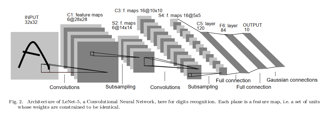
LeNet-5 神经网络一共五层，其中卷积层和池化层可以考虑为一个整体，网络的结构为：

输入 → 卷积 → 池化 → 卷积 → 池化 → 全连接 → 全连接 → 全连接 → 输出。

（2）Pytorch NN Conv2d用法详解

https://blog.csdn.net/HiWangWenBing/article/details/121051650

（3）Pytorch NN MaxPool2d用法详解

https://blog.csdn.net/HiWangWenBing/article/details/121053578

（4）使用Pytorch卷积核构建构建LeNet网络

在 pytorch 中，图像数据集（提供给网络的输入）的存储顺序为：

(batch, channels, height, width)，依次为批大小、通道数、高度、宽度。

å¾2.1 LeNet-5æ¨¡åæ¶æå¾

特别提醒：

LeNet-5网络的默认的输入图片的尺寸是32*32，而Mnist数据集的图片的尺寸是28 * 28。

因此，采用Mnist数据集时，每一层的输出的特征值feature map的尺寸与LeNet-5网络的默认默认的feature map的尺寸是不一样的，需要适当的调整。

具体如何调整，请参考代码的实现：

下面以两种等效的方式定义LeNet神经网络：

Pytorch官网方式
自定义方式

（5）构建LeNet网络结构的代码实例 - 官网

# 来自官网
class LeNet5A(nn.Module):
    def __init__(self):
        super(LeNet5A, self).__init__()
        # 1 input image channel, 6 output channels, 5x5 square convolution kernel
        self.conv1 = nn.Conv2d(in_channels = 1, out_channels = 6,  kernel_size = 5)   # 6 * 24 * 24
        self.conv2 = nn.Conv2d(in_channels = 6, out_channels = 16, kernel_size = 5)   # 16 * 8 * 8
        
        # an affine operation: y = Wx + b
        self.fc1 = nn.Linear(in_features = 16 * 4 * 4, out_features= 120)             # 16 * 4 * 4
        self.fc2 = nn.Linear(in_features = 120, out_features = 84)
        self.fc3 = nn.Linear(in_features = 84,  out_features = 10)

    def forward(self, x):
        # Max pooling over a (2, 2) window
        x = F.max_pool2d(F.relu(self.conv1(x)), (2, 2))
        # If the size is a square, you can specify with a single number
        x = F.max_pool2d(F.relu(self.conv2(x)), 2)
        
        x = torch.flatten(x, 1) # flatten all dimensions except the batch dimension
        x = F.relu(self.fc1(x))
        x = F.relu(self.fc2(x))
        x = self.fc3(x)
        #x = F.log_softmax(x,dim=1)
        return x

（6）构建LeNet网络结构的代码实例 - 自定义

class LeNet5B(nn.Module):
    def __init__(self):
        super(LeNet5B, self).__init__()
        
        self.feature_convnet = nn.Sequential(OrderedDict([
            ('conv1', nn.Conv2d (in_channels = 1, out_channels = 6, kernel_size= (5, 5), stride = 1)),   # 6 * 24 * 24
            ('relu1', nn.ReLU()),
            ('pool1', nn.MaxPool2d(kernel_size=(2, 2))),                                                 # 6 * 12 * 12
            ('conv2', nn.Conv2d (in_channels = 6, out_channels = 16, kernel_size=(5, 5))),               # 16 * 8 * 8
            ('relu2', nn.ReLU()),
            ('pool2', nn.MaxPool2d(kernel_size=(2, 2))),                                                 # 16 * 4 * 4
        ]))

        self.class_fc = nn.Sequential(OrderedDict([
            ('fc1', nn.Linear(in_features = 16 * 4 * 4, out_features = 120)),     # 16 * 4 * 4
            ('relu3', nn.ReLU()),
            ('fc2', nn.Linear(in_features = 120, out_features = 84)),     
            ('relu4', nn.ReLU()),
            ('fc3', nn.Linear(in_features = 84, out_features = 10)),
        ]))

    def forward(self, img):
        output = self.feature_convnet(img)
        output = output.view(-1, 16 * 4 * 4)   #相当于Flatten()
        output = self.class_fc(output)
        return output