


Hybrid A*
Workflow
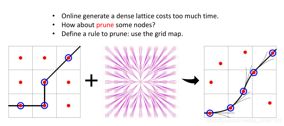
T: 将栅格地图的路径搜索与lattice grid 结合起来 ,保证在每个栅格里面只有一个状态(节点),如下图所示
Y:在线生成密集的栅格花费太多的时间。
算法提出[论文]
(Practical Search Techniques in Path Planning for Autonomous Driving , Dmitri Y:Dolgov , Sebastian Thrun
Path Planning for Autonomous Vehicles in Unknown Semi-structured Environments, Dmitri Dolgov , Sebastian
Detail
维护一个优先队列来存储所有要扩展的节点
•所有节点的启发式函数h(n)是预先定义的
•优先队列初始化为启动状态X S
•对图中所有其他节点赋值g(X S)=0, g(n)=infinite
•循环
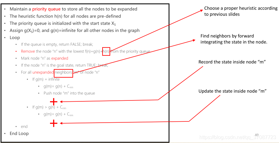
与A四面八方寻找不同,hybrid A是控制输入演化的邻居节点
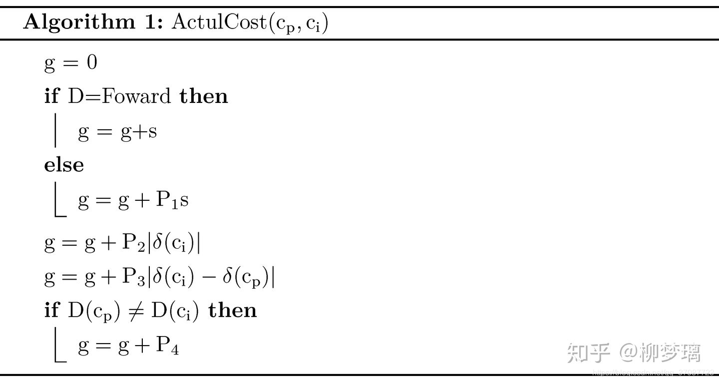
在Hybrid A Star就考虑很多其他因素,比如说转向角转向角的改变,是否倒车,车辆行驶方向是否改变等。如果用
δ
\delta
δ表示车辆的转向角,D表示车辆的行驶方向,s表示每次搜索所走的路程。下图是该计算实际花费的过程,
P
1
−
P
4
P_1-P_4
P1−P4是参数。
Heuristic design
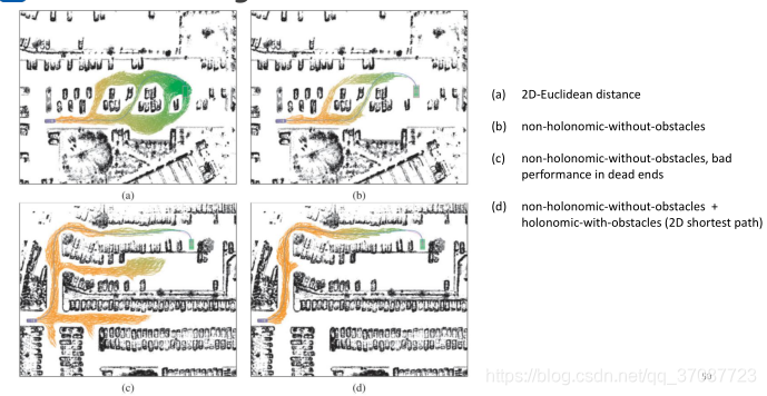
(a) 二维欧式距离
(b)考虑车辆模型,运动学(不能够侧滑)
(c)走入死胡同
(d)考虑障碍物,在2D地图上找最短路径
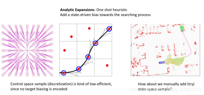
trick
one-shot
分析扩展:一次启发式加上状态驱动对搜索过程的偏重
尝试去查找树,探寻到终点的路径
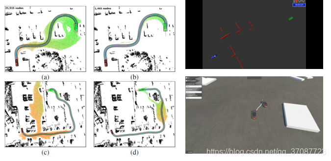
Application
Practical Search Techniques in Path Planning for Autonomous Driving , Dmitri Dolgov , Sebastian
高飞老师的工作
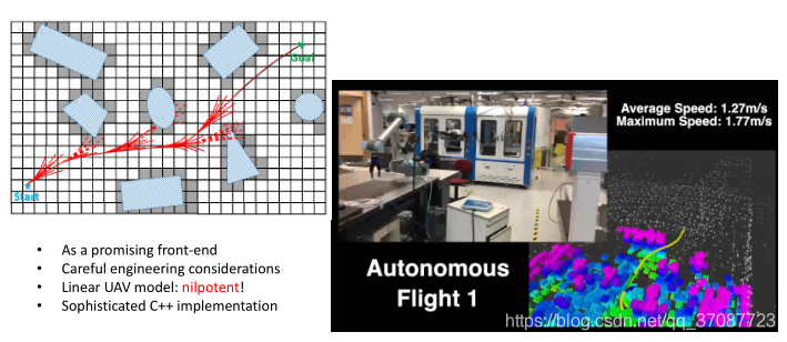
Robust and Efficient Quadrotor Trajectory Generation for Fast Autonomous Flight , Boyu Zhou, Fei Gao
源码
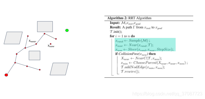
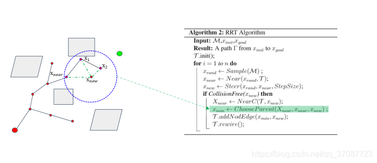
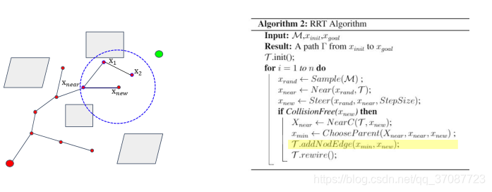
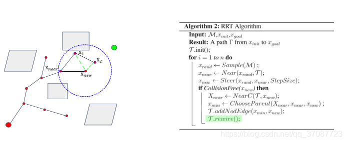
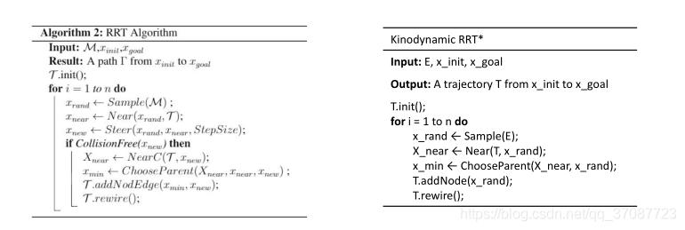
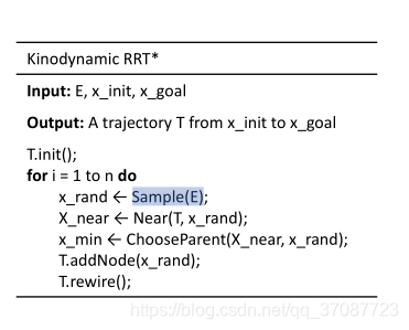
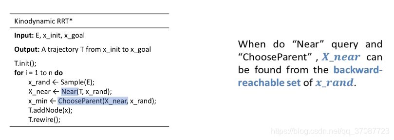
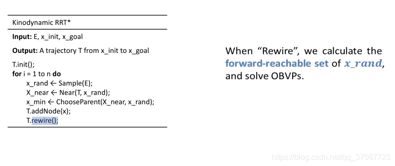
Kinodynamic RRT*
Review:RRT*
 OBVP问题求解
O
RRT vs RRT*
Problems when it comes to motion constraints(运动约束问题)
How to sample
状态空间扩展,系统变量包含位置和速度
How to define “Near”
如果没有运动约束,可以使用欧几里得距离或曼哈顿距离。
而在有运动约束的状态空间中,引入最优控制。
如果引入最优控制,我们可以得到状态间转移的代价函数。
通常考虑能量与时间最优,如果从一种状态转移到另一种状态的成本很小,则两种状态是接近的。(注意,如果反向转移,成本可能不同),如果我们知道到达时间(
τ
\tau
τ)和控制策略
u
(
t
)
u\left( t \right)
u(t)的转移,我们可以计算成本。这些都是经典的最优控制解。
- 固定最终状态,最后时间
最优控制策略 u ∗ ( t ) u^*\left( t \right) u∗(t)
u ∗ ( t ) = R − 1 B T exp [ A T ( τ − t ) ] G ( τ ) − 1 [ x 1 − x ˉ ( τ ) ] u^*\left( t \right) =R^{-1}B^T\exp \left[ A^T\left( \tau -t \right) \right] G\left( \tau \right) ^{-1}\left[ x_1-\bar{x}\left( \tau \right) \right] u∗(t)=R−1BTexp[AT(τ−t)]G(τ)−1[x1−xˉ(τ)]
G(t)为可加权可控格兰姆行列式
G
˙
(
t
)
=
A
G
(
t
)
+
G
(
t
)
A
T
+
B
R
−
1
B
T
,
G
(
0
)
=
0.
\dot{G}\left( t \right) =\mathrm{AG}\left( \mathrm{t} \right) +\mathrm{G}\left( \mathrm{t} \right) \mathrm{A}^{\mathrm{T}}+\mathrm{BR}^{-1}\mathrm{B}^{\mathrm{T}},\mathrm{G}\left( 0 \right) =0.
G˙(t)=AG(t)+G(t)AT+BR−1BT,G(0)=0.
也就是李雅普诺夫方程的解
G
˙
(
t
)
=
A
G
(
t
)
+
G
(
t
)
A
T
+
B
R
−
1
B
T
,
G
(
0
)
=
0.
\dot{G}\left( t \right) =\mathrm{AG}\left( \mathrm{t} \right) +\mathrm{G}\left( \mathrm{t} \right) \mathrm{A}^{\mathrm{T}}+\mathrm{BR}^{-1}\mathrm{B}^{\mathrm{T}},\mathrm{G}\left( 0 \right) =0.
G˙(t)=AG(t)+G(t)AT+BR−1BT,G(0)=0.
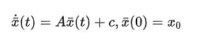
x
ˉ
(
t
)
\bar{x}\left(t\right)
xˉ(t)在t时刻没有控制输入作用下的状态
x
x
x
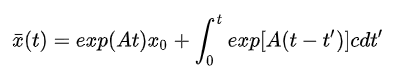
微分方程的解为
- 固定最终状态x1,对最终时间τ不加限制
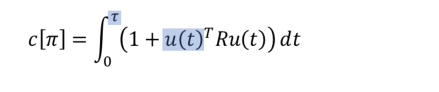
如果我们想要找到最佳的到达时间( t t t),为此,我们确定控制策略 u ∗ ( t ) u^*\left(t\right) u∗(t)的成本函数( c [ π ] c\left[\pi\right] c[π])和评估积分
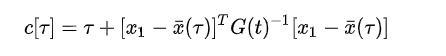
找到最优( τ \tau τ)通过( c [ τ ] c\left[\tau\right] c[τ])对 τ \tau τ的微分
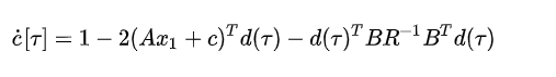
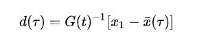
解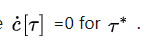
注意,函数( c [ τ ] c\left[\tau\right] c[τ])可能有多个局部最小值。双积分器系统,这是一个( 4 t h 4^{th} 4th)阶多项式。
给出最优到达时间 τ ∗ \tau^* τ∗正如上面定义的,又变成了一个固定的最终状态。修正了最终时间问题。
How to “chooseParent”
现在如果我们对一个随机状态进行抽样,我们就可以从树中的这些状态节点计算出控制策略和到抽样状态代价,选择一个以最小的成本和检查(
x
(
t
)
x(t)
x(t)]和(
u
(
t
)
u(t)
u(t)范围。
如果没有找到合格的父节点,则对另一个状态进行取样。
How to find near nodes efficiently
查找一部分空间
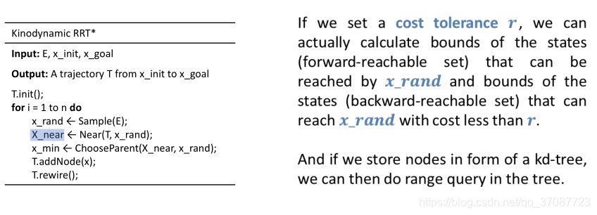
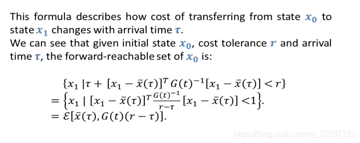
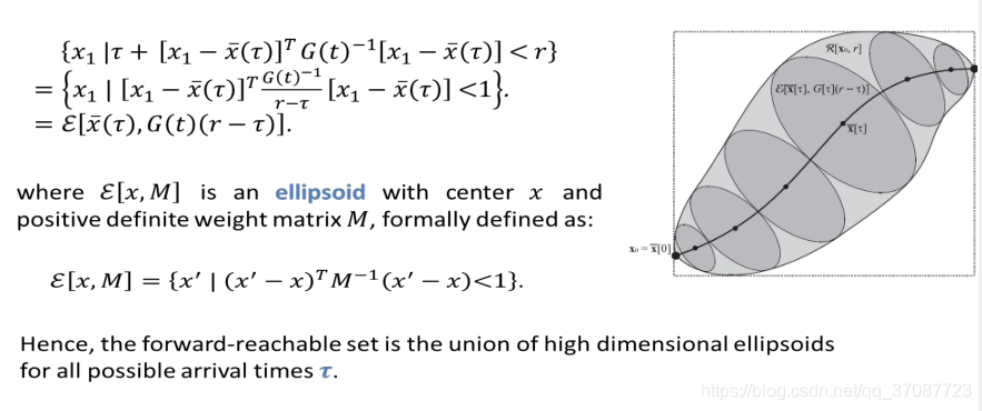
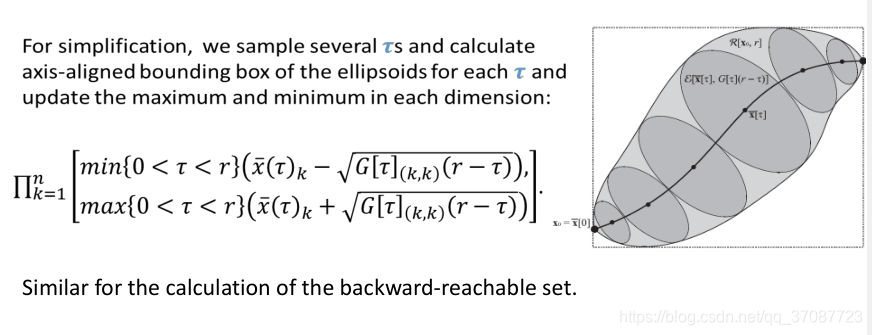
如果我们设置一个成本容忍度r,我们可以计算实际状态的界(前向可达集),其能通过x_rand和状态界(反向可达集)得到。以低于r的成本到达x_rand。
如果我们以kd树的形式存储节点,我们可以在树中进行范围查询。
c
[
τ
]
=
τ
+
[
x
1
−
x
ˉ
(
τ
)
]
T
G
(
t
)
−
1
[
x
1
−
x
ˉ
(
τ
)
]
\mathrm{c}\left[ \mathrm{\tau} \right] =\mathrm{\tau}+\left[ \mathrm{x}_1-\mathrm{\bar{x}}\left( \mathrm{\tau} \right) \right] ^{\mathrm{T}}\mathrm{G}\left( \mathrm{t} \right) ^{-1}\left[ \mathrm{x}_1-\mathrm{\bar{x}}\left( \mathrm{\tau} \right) \right]
c[τ]=τ+[x1−xˉ(τ)]TG(t)−1[x1−xˉ(τ)]
How to “rewire”
计算前向可达集
演示
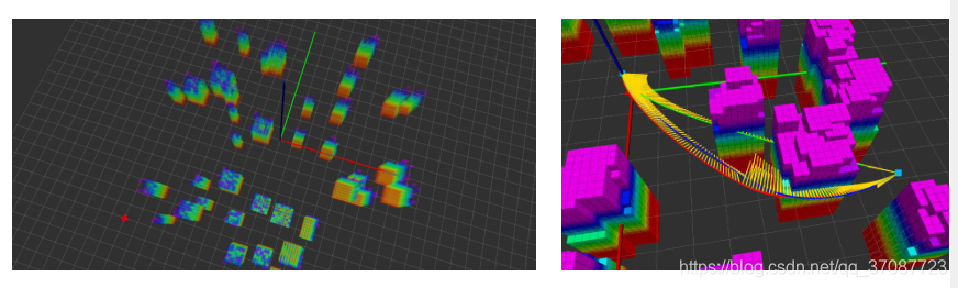
绿色曲线不考虑障碍;
红色曲线是考虑动力kinodynamic轨迹规划器的结果;
蓝色曲线为运动学轨迹规划器找到的第一个可行轨迹;
黄线是每个控制点的控制输入。
Homework
- 假设位置是固定的,速度和加速度在这里是不加限制的,如何扩展邻居?
根据前面提到的OBVP,求得部分自由最终状态情况的最优解(控制、状态、时间)。 - 建立一个线性机器人模型的ego-graph(由唯一一个中心节点(ego),以及这个节点的邻居(alters)组成)编程生成许多个轨迹,设计一个打分函数,选择最接近规划目标的最佳轨迹,如演示图那样。


 1483
1483

 被折叠的 条评论
为什么被折叠?
被折叠的 条评论
为什么被折叠?
 到【灌水乐园】发言


