导入必要的包
suppressPackageStartupMessages(library(PseudotimeDE))
suppressPackageStartupMessages(library(SingleCellExperiment))
suppressPackageStartupMessages(library(slingshot))
suppressPackageStartupMessages(library(tibble))
suppressPackageStartupMessages(library(dplyr))
suppressPackageStartupMessages(library(scales))
导入 Seurat 对象并预处理
load("./processfile/S01-osi-Seurat.RData")
if(T){
  sce <- NormalizeData(object = sce, scale.factor = 1e6)
  sce <- FindVariableFeatures(object = sce)
  sce <- ScaleData(object = sce)
}
提取标准化表达谱和PCA数据
# 提取标准化表达谱后进行降维
norms <- as.matrix(t(sce@assays$RNA@data)) %>% t()
rd = sce@reductions$pca@cell.embeddings[,1:2]
转换为SingleCellExperiment对象
pt.obj <- SingleCellExperiment(
  assays = list(norms = norms),
  meta = list(metadata = sce@meta.data),
  reducedDims = SimpleList(PCA = rd)
  )
计算伪时间
colData(pt.obj)$cl <- pt.obj@metadata$metadata$prelabel # 分组信息

# 计算伪时间值
fit_ori <- slingshot(pt.obj, reducedDim = 'PCA', clusterLabels = "prelabel")
pt.obj_ori_tbl <- tibble(cell = colnames(pt.obj), pseudotime = scales::rescale(colData(fit_ori)$slingPseudotime_1))

# 计算伪时间图谱

res_fix <- PseudotimeDE::runPseudotimeDE(gene.vec = c("CCL5", "CXCL10"),
                                     ori.tbl = pt.obj_ori_tbl,
                                     sub.tbl = NULL, # Set as NULL to only get fix.pv
                                     sce = pt.obj,
                                     model = "nb")

# 可视化
PseudotimeDE::plotCurve(gene.vec = res_fix$gene,
                                        ori.tbl = pt.obj_ori_tbl,
                                        sce = pt.obj,
                                        model.fit = res_fix$gam.fit)
整合成函数后方便直接调用
options(mc.cores = 12)
seurat.pseudotime = function(sce,gene_list,group,sub.tbl = NULL){
pt.obj = SingleCellExperiment(
assays = list(norms = as.matrix(sce@assays$RNA@data),
counts = as.matrix(sce@assays$RNA@counts)),
meta = list(metadata = sce@meta.data),
reducedDims = SimpleList(PCA = sce@reductions$pca@cell.embeddings[,1:2])
)
gc()
colData(pt.obj)$prelabel <- pt.obj@metadata$metadata[group][,1]
fit_ori <- slingshot(pt.obj, reducedDim = 'PCA', clusterLabels = "prelabel")
pt.obj_ori_tbl <- tibble(cell = colnames(pt.obj), pseudotime = scales::rescale(colData(fit_ori)$slingPseudotime_1))
gc()
res_fix <- PseudotimeDE::runPseudotimeDE(gene.vec = gene_list,
ori.tbl = pt.obj_ori_tbl,
sub.tbl = NULL,
sce = pt.obj,
model = 'nb')
stopifnot(is.list(res_fix$gam.fit))
stopifnot(length(res_fix$gene) == length(res_fix$gam.fit))
cell <- gene <- ori_pseudotime <- pseudotimes <- pseudotime <- counts <- NULL
pt.obj <- pt.obj[, pt.obj_ori_tbl$cell]
count_mat <- assays(pt.obj)$counts
count_mat <- cbind(t(count_mat), pseudotime = pt.obj_ori_tbl$pseudotime)
count_mat = cbind(count_mat,group = colData(pt.obj)$prelabel)
count_mat <- count_mat %>% as_tibble() %>% tidyr::pivot_longer(cols = res_fix$gene,
names_to = "gene", values_to = "counts") %>% dplyr::select(gene,
pseudotime, counts,group)
dat <- mapply(X = res_fix$gene, Y = res_fix$gam.fit, function(X, Y) {
count_mat %>% dplyr::filter(gene == X) %>% dplyr::mutate(fitted = predict(Y,
type = "response"))
}, SIMPLIFY = FALSE)
dat <- dplyr::bind_rows(dat)
dat$pseudotime = as.numeric(dat$pseudotime)
dat$counts = as.numeric(dat$counts)
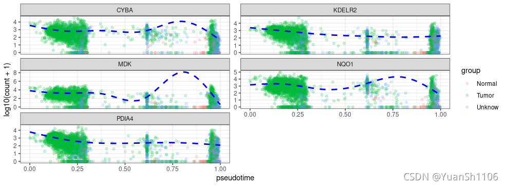
p <- dat %>% ggplot(aes(x = pseudotime, y = log10(counts + 1),color = group)) + geom_point(alpha = 0.2) + facet_wrap(~gene,
ncol = 2, scales = "free_y") + ylab("log10(count + 1)") +
geom_line(aes(y = log10(fitted + 1)), col = "blue", lty = "dashed",
size = 1) + theme_bw()
p
}
gene_list = read.csv('./111.csv')[,1]
seurat.pseudotime(sce,gene_list[1:5],'prelabel')
使用方法
seurat.pseudotime(sce,gene_list[1:5],'prelabel')


 1万+
1万+

 被折叠的 条评论
为什么被折叠?
被折叠的 条评论
为什么被折叠?
 到【灌水乐园】发言


