单细胞聚类，究竟聚类聚成多少类比较合适？全代码分享

最新推荐文章于 2025-02-22 19:31:13 发布

生信小博士

最新推荐文章于 2025-02-22 19:31:13 发布

阅读量2.4k

点赞数 15

文章标签：聚类算法数据挖掘

本文链接：https://blog.csdn.net/qq_52813185/article/details/134027916

版权

单细胞数据分析到最后一步往往都需要聚类，进而给亚群命名。但是我们通常纠结resolution到底选多大为好，究竟聚成多少类比较合适？今天我们使用Silhouette来确定多少类比较合适。

关注微信：生信小博士

选择最优聚类有多种方式，今天着重于Silhouette Method。

Determining optimal number of clusters (k)

Before we do the actual clustering, we need to identity the Optimal number of clusters (k) for this data set of wholesale customers. The popular way of determining number of clusters are

Elbow Method
Silhouette Method
Gap Static Method

Elbow and Silhouette methods are direct methods and gap statistic method is the statistics method.

In this demonstration, we are going to see how silhouette method is used.

1 最优聚类数据前处理

如果你已经准备好前期的数据，此步可以省略。

这一步的目的：会得到一个名为inttegtaed_data的seurat对象。

slide_files <- list.files("~/silicosis/spatial/prcessed_visum_for_progeny/data/",recursive = TRUE,
                                        all.files = TRUE,full.names = TRUE,pattern = "_")




integrated_data <- map(slide_files, readRDS)
print("You managed to load everything")
print("Object size")
print(object.size(integrated_data))





# Calculate HVG per sample - Here we assume that batch and patient effects aren't as strong
# since cell-types and niches should be greater than the number of batches

Assays(integrated_data [[1]])
str(integrated_data [[1]])



def_assay="Spatial"


hvg_list <- map(integrated_data, function(x) {
  
  DefaultAssay(x) <- def_assay
  
  x <- FindVariableFeatures(x, selection.method = "vst", 
                            nfeatures = 3000)
  
  x@assays[[def_assay]]@var.features
  
}) %>% unlist()

hvg_list <- table(hvg_list) %>%
  sort(decreasing = TRUE)




gene_selection_plt <- hvg_list %>% enframe() %>% 
  group_by(value) %>% 
  mutate(value = as.numeric(value)) %>%
  summarize(ngenes = length(name)) %>% 
  ggplot(aes(x = value, y = ngenes)) + 
  geom_bar(stat = "identity")

gene_selection <- hvg_list[1:3000] %>% names()


#########
# Create merged object ---------------------------------
integrated_data <- purrr::reduce(integrated_data,
                          merge,
                          merge.data = TRUE)

print("You managed to merge everything")
print("Object size")
print(object.size(integrated_data))

# Default assay ---------------------------------------
#DefaultAssay(integrated_data) <- def_assay



# Process it before integration -----------------------
integrated_data <- integrated_data %>%
  ScaleData(verbose = FALSE) %>% 
  RunPCA(features = gene_selection, 
         npcs = 30, 
         verbose = FALSE) 

original_pca_plt <- DimPlot(object = integrated_data, 
                            reduction = "pca", 
                            pt.size = .1, 
                            group.by = "orig.ident")

head(integrated_data@meta.data)

batch_covars="orig.ident"
# Integrate the data -----------------------
integrated_data <- RunHarmony(integrated_data, 
                              group.by.vars =   batch_covars, 
                              plot_convergence = TRUE,
                              assay.use = def_assay,
                              max.iter.harmony = 20)



# Corrected dimensions -----------------------
corrected_pca_plt <- DimPlot(object = integrated_data, 
                             reduction = "harmony", 
                             pt.size = .1, 
                             group.by = "orig.ident")


# Create the UMAP with new reduction -----------
integrated_data <- integrated_data %>% 
  RunUMAP(reduction = "harmony", dims = 1:30,
          reduction.name = "umap_harmony") %>%
  RunUMAP(reduction = "pca", dims = 1:30,
          reduction.name = "umap_original")

integrated_data <- FindNeighbors(integrated_data, 
                                 reduction = "harmony", 
                                 dims = 1:30)

head(integrated_data@meta.data)

colnames(integrated_data@meta.data)=gsub(pattern ="_snn_res.",replacement = "_before",x = colnames(integrated_data@meta.data) )

准备好的数据如下。这里的数据你可以使用seurat的pbmc教程中的数据，作为练习。

然后进行下一步

2 开始最优聚类

全代码如下

optimize=TRUE
################opt cluster--------------
if(optimize) { 
  
  # Clustering and optimization -------------------------
  print("Optimizing clustering")
  
  seq_res <- seq(0.5, 1.5, 0.1)
  
# seq_res=1
  integrated_data <- FindClusters(integrated_data,
                                  resolution = seq_res,
                                  verbose = F)
  
  clustree_plt <- clustree::clustree(integrated_data, 
                           prefix = paste0(DefaultAssay(integrated_data), "_snn_res."))
  
  # Optimize clustering ------------------------------------------------------
  cell_dists <- dist(integrated_data@reductions$harmony@cell.embeddings,
                     method = "euclidean")
  head(cell_dists)
 
  
  cluster_info <- integrated_data@meta.data[,grepl(paste0(DefaultAssay(integrated_data),"_snn_res"),
                                                   colnames(integrated_data@meta.data))] %>%
    dplyr::mutate_all(as.character) %>%
    dplyr::mutate_all(as.numeric)
  
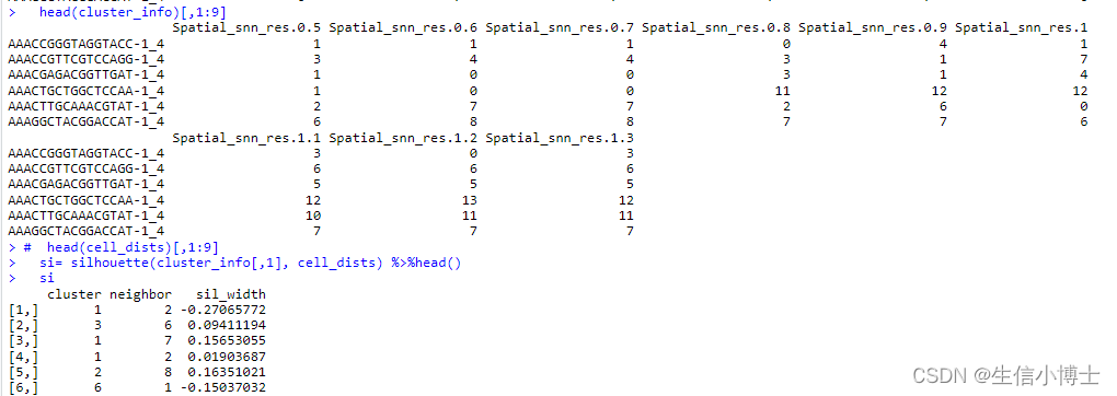
  head(cluster_info)[,1:9]
#  head(cell_dists)[,1:9]
  si= silhouette(cluster_info[,1], cell_dists) %>%head()
  si
   
  silhouette_res <- apply(cluster_info, 2, function(x){
    si <- silhouette(x, cell_dists)
   
     if(!any(is.na(si))) {
      mean(si[, 'sil_width'])
    } else {
      NA
    }
  })
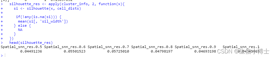
  head(silhouette_res)
  
  integrated_data[["opt_clust_integrated"]] <- integrated_data[[names(which.max(silhouette_res))]]
  
  Idents(integrated_data) = "opt_clust_integrated"

最终会得到一个opt_clust_integrated，代表最优聚类的清晰度。如果你的数据比较大，可以调整 seq_res <- seq(0.5, 1.5, 0.1)，把1.5调到3，甚至更高。

上述代码的部分运行结果：

根据下面的图，resolution为0.7是最优聚类

3 找到最优聚类之后，把多余的聚类结果删掉，节省内存

全代码如下

  # Reduce meta-data -------------------------------------------------------------------------
  spam_cols <- grepl(paste0(DefaultAssay(integrated_data), "_snn_res"),
                     colnames(integrated_data@meta.data)) |
    grepl("seurat_clusters",colnames(integrated_data@meta.data))
  
  integrated_data@meta.data <- integrated_data@meta.data[,!spam_cols]
  
} else {
  
  print("Not Optimizing clustering")
  
  seq_res <- seq(0.2, 1.6, 0.2)
  
  integrated_data <- FindClusters(integrated_data,
                                  resolution = seq_res,
                                  verbose = F)
  
  clustree_plt <- clustree(integrated_data, 
                           prefix = paste0(DefaultAssay(integrated_data), 
                                           "_snn_res."))
  
  integrated_data <- FindClusters(integrated_data,
                                  resolution = default_resolution,
                                  verbose = F)
  
  integrated_data[["opt_clust_integrated"]] <- integrated_data[["seurat_clusters"]]
  
  spam_cols <- grepl(paste0(DefaultAssay(integrated_data), "_snn_res"),
                     colnames(integrated_data@meta.data)) |
    grepl("seurat_clusters",colnames(integrated_data@meta.data))
  
  integrated_data@meta.data <- integrated_data@meta.data[,!spam_cols]
  
}

4 保存对象

# Save object ------------------------------------------------------
saveRDS(integrated_data, file ="~/silicosis/spatial/integrated_slides/integrated_slides.rds" )

关注微信：生信小博士

参考：

https://medium.com/codesmart/r-series-k-means-clustering-silhouette-794774b46586#id_token=eyJhbGciOiJSUzI1NiIsImtpZCI6ImEwNmFmMGI2OGEyMTE5ZDY5MmNhYzRhYmY0MTVmZjM3ODgxMzZmNjUiLCJ0eXAiOiJKV1QifQ.eyJpc3MiOiJodHRwczovL2FjY291bnRzLmdvb2dsZS5jb20iLCJhenAiOiIyMTYyOTYwMzU4MzQtazFrNnFlMDYwczJ0cDJhMmphbTRsamRjbXMwMHN0dGcuYXBwcy5nb29nbGV1c2VyY29udGVudC5jb20iLCJhdWQiOiIyMTYyOTYwMzU4MzQtazFrNnFlMDYwczJ0cDJhMmphbTRsamRjbXMwMHN0dGcuYXBwcy5nb29nbGV1c2VyY29udGVudC5jb20iLCJzdWIiOiIxMTIyMzMxNDE1MDU0MDY1NzA5OTMiLCJlbWFpbCI6ImFudGkuY2FuY2VyLmZpZ2h0ZXJAZ21haWwuY29tIiwiZW1haWxfdmVyaWZpZWQiOnRydWUsIm5iZiI6MTY5ODE5ODYzMCwibmFtZSI6InlhbmcgeWFuZyIsInBpY3R1cmUiOiJodHRwczovL2xoMy5nb29nbGV1c2VyY29udGVudC5jb20vYS9BQ2c4b2NKUjVFOGJoU2wxRUVtUDcyVXhPUExGU2VlNlcza2hlZVItVnVaZDZiei09czk2LWMiLCJnaXZlbl9uYW1lIjoieWFuZyIsImZhbWlseV9uYW1lIjoieWFuZyIsImxvY2FsZSI6ImVuIiwiaWF0IjoxNjk4MTk4OTMwLCJleHAiOjE2OTgyMDI1MzAsImp0aSI6ImJlNjYyNmYyMWMwZGE4MjgzZWUzMWEzMGU0ZGY2MWQ0Y2M3YzlkODgifQ.FddjhGbYiuFDFjWFmjGcAXNdbuR3XyqzqWWv8NvyJnREj48qhcFsI4HHv0DWnwewOsmr2jnCnC51nInSyBvgZJSjAQMdUAVpoZTwvroliR3wB6q8In29eXhZ2N_WgqVqoTcMT5yECF4oJrVZgDYxG5t17KAIYso3pvbpCy-5oVq8zBPZ8M8HRd83upKAODDC4bAKtGsGqlFYDV-bD7L1pXsRw3HWebcyY7bfk74FVtnveGyk-A0VIHjDIAdxxjqMiZmuntRX7PUV-nXhSeiBxzI8W4kjHO8uQKlwaCgjyOARTNQ2b-AOY5f5gr6BP0kin9DN6rk7QuPfrvVIgg4yGwhttps://medium.com/codesmart/r-series-k-means-clustering-silhouette-794774b46586#id_token=eyJhbGciOiJSUzI1NiIsImtpZCI6ImEwNmFmMGI2OGEyMTE5ZDY5MmNhYzRhYmY0MTVmZjM3ODgxMzZmNjUiLCJ0eXAiOiJKV1QifQ.eyJpc3MiOiJodHRwczovL2FjY291bnRzLmdvb2dsZS5jb20iLCJhenAiOiIyMTYyOTYwMzU4MzQtazFrNnFlMDYwczJ0cDJhMmphbTRsamRjbXMwMHN0dGcuYXBwcy5nb29nbGV1c2VyY29udGVudC5jb20iLCJhdWQiOiIyMTYyOTYwMzU4MzQtazFrNnFlMDYwczJ0cDJhMmphbTRsamRjbXMwMHN0dGcuYXBwcy5nb29nbGV1c2VyY29udGVudC5jb20iLCJzdWIiOiIxMTIyMzMxNDE1MDU0MDY1NzA5OTMiLCJlbWFpbCI6ImFudGkuY2FuY2VyLmZpZ2h0ZXJAZ21haWwuY29tIiwiZW1haWxfdmVyaWZpZWQiOnRydWUsIm5iZiI6MTY5ODE5ODYzMCwibmFtZSI6InlhbmcgeWFuZyIsInBpY3R1cmUiOiJodHRwczovL2xoMy5nb29nbGV1c2VyY29udGVudC5jb20vYS9BQ2c4b2NKUjVFOGJoU2wxRUVtUDcyVXhPUExGU2VlNlcza2hlZVItVnVaZDZiei09czk2LWMiLCJnaXZlbl9uYW1lIjoieWFuZyIsImZhbWlseV9uYW1lIjoieWFuZyIsImxvY2FsZSI6ImVuIiwiaWF0IjoxNjk4MTk4OTMwLCJleHAiOjE2OTgyMDI1MzAsImp0aSI6ImJlNjYyNmYyMWMwZGE4MjgzZWUzMWEzMGU0ZGY2MWQ0Y2M3YzlkODgifQ.FddjhGbYiuFDFjWFmjGcAXNdbuR3XyqzqWWv8NvyJnREj48qhcFsI4HHv0DWnwewOsmr2jnCnC51nInSyBvgZJSjAQMdUAVpoZTwvroliR3wB6q8In29eXhZ2N_WgqVqoTcMT5yECF4oJrVZgDYxG5t17KAIYso3pvbpCy-5oVq8zBPZ8M8HRd83upKAODDC4bAKtGsGqlFYDV-bD7L1pXsRw3HWebcyY7bfk74FVtnveGyk-A0VIHjDIAdxxjqMiZmuntRX7PUV-nXhSeiBxzI8W4kjHO8uQKlwaCgjyOARTNQ2b-AOY5f5gr6BP0kin9DN6rk7QuPfrvVIgg4yGw