


机器学习 人类学习

什么是主动学习? (What is Active Learning?)
Active Learning is a sub-field of Machine Learning wherein the model can query the user for desired information as the training process progresses. The user (or the Oracle) then labels the required data and adds it to the training samples. This way, the model can learn by active interaction with a human and unnecessary data structuring and annotations can be avoided.
主动学习是机器学习的子领域,其中,随着训练过程的进行,模型可以向用户查询所需的信息。 然后,用户(或Oracle)标记所需的数据并将其添加到训练样本中。 这样,模型可以通过与人类的主动交互来学习,并且可以避免不必要的数据结构,并且可以避免注释。
This article aims at explaining the logic of active learning along with an example with the IMDB Sentiment Analysis dataset and Tensorflow 2.x
本文旨在说明主动学习的逻辑以及IMDB情感分析数据集和Tensorflow 2.x的示例
主动学习如何工作?(How does Active Learning work?)
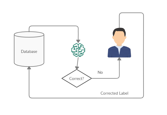
Active Learning is an active region of research where you start by labelling a small amout of data from your pool of unlablled data, fit a model to this small dataset and predict on a stratified test dataset to obtain the model’s uncertanities. The user (or Oracle) then labels another part of the unlabelled pool consisting of samples which the model is the most uncertain about. This is added back to the dataset and the training is continued. This process is repeated till the model achieves the desired entropy score after which it is sent to the deployment stage. The use case of active learning is important in today’s world as manually annotating the data can be expensive as well as exhausting.
主动学习是一个活跃的研究区域,你从你的unlablled数据池标签数据的一个小量开始,拟合模型这个小数据集,并预测在分层测试数据集来获得模型的uncertanities。 然后,用户(或Oracle)标记未标记池的另一部分,该部分由模型最不确定的样本组成。 这将添加回数据集中,并且训练将继续。 重复此过程,直到模型达到所需的熵值,然后将其发送到部署阶段。 主动学习的用例在当今世界中很重要,因为手动注释数据既昂贵又费力。
让我们开始吧! (Lets get started!)
At this point, some code will provide better understanding to the theory above. We will use the IMDB dataset along with a very basic tf.keras model to demonstrate the usage of active learning for real life scenarios.
在这一点上,一些代码将更好地理解上述理论。 我们将使用IMDB数据集以及一个非常基本的tf.keras模型来演示主动学习在现实生活场景中的用法。
import tensorflow as tf
import numpy as np
import re, os
import matplotlib.pyplot as plt
import pandas as pd
import sklearn
Loading the data from kaggle into our colab environment
将数据从kaggle加载到我们的colab环境中
!mkdir -p ~/.kaggle
!cp kaggle.json ~/.kaggle/
!chmod 600 /root/.kaggle/kaggle.json
!kaggle datasets download -d columbine/imdb-dataset-sentiment-analysis-in-csv-format
!unzip '/content/imdb-dataset-sentiment-analysis-in-csv-format.zip'
Reading the dataset as a pandas DataFrame and checking the split
将数据集作为pandas DataFrame读取并检查拆分
df_train = pd.read_csv('/content/Train.csv')
df_val = pd.read_csv('/content/Valid.csv')
df_test = pd.read_csv('/content/Test.csv')


df_train['label'].value_counts()


# 0-> 20019
# 1-> 19981
Cleaning the Dataset. We remove all tags, excessive repetition of characters and unnecessary spaces.
清理数据集。 我们删除了所有标签,过多的字符重复和不必要的空格。
# Cleaning/Preprocessing Helper function


def preprocess(s):
  s = re.sub(r'@[a-zA-Z0-9_.]+ ', '', str(s))
  s = re.sub(r'#[a-zA-Z0-9_.]+ ', '', str(s))
  s = re.sub(r'''[^a-zA-Z0-9?. ]+''', '', s)
  s = re.sub(r''''[' ']+''', " ", s)
  s = re.sub(r'(\w)\1{2,}',r'\1',s)
  s = s.lower().strip()
  return s


df_train['text'] = df_train['text'].apply(preprocess)
df_val['text'] = df_val['text'].apply(preprocess)
df_test['text'] = df_test['text'].apply(preprocess)
We now split the data into training, testing and validation sets. We have to make sure that the test set is well sampled and stratified so as to minimize bias.
现在,我们将数据分为训练,测试和验证集。 我们必须确保对测试集进行了良好的采样和分层,以最大程度地减少偏差。
def get_data(df):
  zeros, ones = df[df['label']==0], df[df['label']==1]
  zero_text, zero_labels = zeros['text'].to_numpy(), zeros['label'].to_numpy()
  one_text, one_labels = ones['text'].to_numpy(), ones['label'].to_numpy()
  X, Y = np.concatenate((one_text,zero_text)), np.concatenate((one_labels,zero_labels))
  return X,Y


X_train,Y_train = get_data(df_train)
X_val,Y_val = get_data(df_val)
X_test,Y_test = get_data(df_test)
We use tf.keras’s inbuilt Tokenizer to tokenize the sentences. For this example we set our vocabulary size to 3000 words and our maximum padding length to 50. You are free to tweak these values as per your preference.
我们使用tf.keras的内置Tokenizer标记句子。 在此示例中,我们将词汇量设置为3000个单词,将最大填充长度设置为50。您可以根据自己的喜好随意调整这些值。
# Instantiating the Tokenizer and creating sequences
tokenizer = tf.keras.preprocessing.text.Tokenizer(3000,oov_token=1)
tokenizer.fit_on_texts(X_train)
train_seq = tokenizer.texts_to_sequences(X_train)
val_seq = tokenizer.texts_to_sequences(X_val)
test_seq = tokenizer.texts_to_sequences(X_test)


# Padding all sequences
train_seq = tf.keras.preprocessing.sequence.pad_sequences(train_seq,maxlen=50,padding='post')
val_seq = tf.keras.preprocessing.sequence.pad_sequences(val_seq,maxlen=50,padding='post')
test_seq = tf.keras.preprocessing.sequence.pad_sequences(test_seq,maxlen=50,padding='post')定义模型(Defining the Model)
We will be working with a simple sequential model with around 200k parameters as stated below. The model is kept simple so as to ensure quick training.
我们将使用一个具有约200k参数的简单顺序模型,如下所述。 模型保持简单,以确保快速训练。
from tensorflow.keras.layers import Embedding,Dense,LSTM,Flatten,Dropout


def create_model():
  model = tf.keras.models.Sequential()
  model.add(Embedding(3000,64))
  model.add(LSTM(32))
  model.add(Flatten())
  model.add(Dense(64,activation='relu'))
  model.add(Dropout(0.3))
  model.add(Dense(32,activation='relu'))
  model.add(Dropout(0.3))
  model.add(Dense(4,activation='relu'))
  model.add(Dense(1,activation='sigmoid'))
  model.summary()
  model.compile(optimizer=tf.keras.optimizers.Adam(0.0001),loss=tf.keras.losses.BinaryCrossentropy(),metrics=['accuracy'])
  return model
Model: "sequential_1" _________________________________________________________________ Layer (type) Output Shape Param # ================================================================= embedding_1 (Embedding) (None, None, 64) 192000 _________________________________________________________________ lstm_1 (LSTM) (None, 32) 12416 _________________________________________________________________ flatten_1 (Flatten) (None, 32) 0 _________________________________________________________________ dense_4 (Dense) (None, 64) 2112 _________________________________________________________________ dropout_2 (Dropout) (None, 64) 0 _________________________________________________________________ dense_5 (Dense) (None, 32) 2080 _________________________________________________________________ dropout_3 (Dropout) (None, 32) 0 _________________________________________________________________ dense_6 (Dense) (None, 4) 132 _________________________________________________________________ dense_7 (Dense) (None, 1) 5 ================================================================= Total params: 208,745
Trainable params: 208,745
Non-trainable params: 0训练循环 (Training Loop)
The training procedure of the model consists of:
该模型的训练过程包括:
- First fit on the initial training data 首先适合初始训练数据
- Restoring the model with the best cross-entropy loss恢复具有最佳交叉熵损失的模型
- Predicting using the test set to judge the frequency of incorrect labels使用测试集预测不正确标签的出现频率
- Counting the number of zeros and ones incorrectly classified and finding their ratio计算错误分类的零和一的数目并找到它们的比率
- Sampling data from the pool based on the ratio and appending it to the original data根据比率从池中采样数据并将其附加到原始数据
Continuing training on the new dataset, evaluating and repeating all steps after step 2, N times.
继续对新数据集进行训练,评估并重复步骤2之后的所有步骤N次。
For this example, we are sampling only those data points which are incorrectly classified and adding them to the dataset
在此示例中,我们仅采样那些分类错误的数据点,并将其添加到数据集中
import collections


def train_small_models(train_features,train_labels,pool_features,pool_labels,val_seq,Y_val,test_seq,Y_test,iters=3,sampling_size=5000):


  losses, val_losses, accuracies, val_accuracies = [], [], [], []


  model = create_model()
  checkpoint = tf.keras.callbacks.ModelCheckpoint('Checkpoint.h5',save_best_only=True,verbose=1)


  print(f"Starting to train with {train_features.shape[0]} samples")


  history = model.fit(train_features,train_labels,256,15,validation_data=(val_seq,Y_val),callbacks=[checkpoint,tf.keras.callbacks.EarlyStopping(patience=6,verbose=1)])
  losses, val_losses, accuracies, val_accuracies = append_history(losses,val_losses,accuracies,val_accuracies,history)
  model = tf.keras.models.load_model('Checkpoint.h5')


  for iter_n in range(iters):


    # Getting predictions from previously trained model
    predictions = model.predict(test_seq)
    rounded = np.where(predictions>0.5,1,0)


    # Count number of ones and zeros incorrectly classified
    counter = collections.Counter(Y_test[rounded.squeeze()!=Y_test.squeeze()])


    # Find ratio of ones to zeros. If all samples are correctly classified (Major overfitting) then we set the ratio to 0.5
    if counter[0]!=0 and counter[1]!=0:
      total = counter[0]+counter[1]
      sample_ratio = counter[0]/total if counter[0]>counter[1] else counter[1]/total
    else:
      sample_ratio = 0.5


    sample = np.concatenate((np.random.choice(np.where(pool_labels==0)[0],int(sample_ratio*sampling_size), replace=False),
                             np.random.choice(np.where(pool_labels==1)[0],int(sampling_size*(1-sample_ratio)), replace=False)))
    np.random.shuffle(sample)


    # Get new values from pool
    update_f = pool_features[sample]
    update_l = pool_labels[sample]


    # Remove the chosen samples from pool
    pool_features = np.delete(pool_features,sample,axis=0)
    pool_labels = np.delete(pool_labels,sample)


    # Add the sampled entries to the original data
    train_features = np.vstack((train_features,update_f))
    train_labels = np.hstack((train_labels,update_l))

    print(f"Starting training with {train_features.shape[0]} samples")


    # Retrain the model with the appended data
    history = model.fit(train_features,train_labels,validation_data=(val_seq,Y_val),epochs=15,batch_size=256,callbacks=[checkpoint,tf.keras.callbacks.EarlyStopping(patience=6,verbose=1)])

    losses, val_losses, accuracies, val_accuracies = append_history(losses,val_losses,accuracies,val_accuracies,history)


    model = tf.keras.models.load_model('Checkpoint.h5')
    print(model.evaluate(test_seq,Y_test))


  plot_merged_metrics(losses,val_losses,accuracies,val_accuracies)

  return model
Some other methods of sampling include:
其他一些采样方法包括:
- Entropy based sampling: Sample using a threshold for entropy 基于熵的采样:使用熵阈值进行采样
- Committee based: Train multiple models and sample from the most uncertain predictions基于委员会的:训练多种模型并从最不确定的预测中取样
- Margin Sampling: Exploiting the hyperplane separation for SVMs边距采样:利用SVM的超平面分离
For training the model we have two additional hyperparameters- iters and sampling_size which both can be tweaked freely as they represent the real life scenarios of annotating sampling_size number of data points iter number of times
对于训练模型,我们有两个额外的hyperparameters- iters和sampling_size其中,因为它们代表标注sampling_size的现实生活场景都可以自由调整了 数据点数迭代次数
集合与推理(Ensembling and Inference)
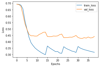
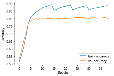
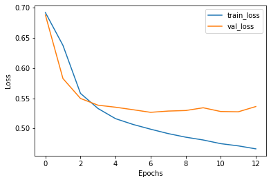
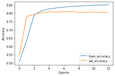
We train three models each for both, the full dataset and the active learning based procedure of sampling. The resultant averaged graphs are as follows:
我们为完整的数据集和基于主动学习的抽样程序都训练了三个模型。 所得的平均图如下:
Final scores for the model ensembles are:
模型合奏的最终成绩为:
Passive Learning on 40,000 sentences
Accuracy: 0.8224
Precision: 0.8339
Recall: 0.8156Active Learning on 30,000 sentences
Accuracy: 0.8152
Precision: 0.8387
Recall: 0.8016
As we can see from the scores, Active Learning method performs equally as good if not better than Passive Learning. Active Learning requires only 30,000 samples to reach the same score as the one Passive Learning achieves on 40,000 samples. The feature of not having to annotate all data at once saves both time and money for the company.
从分数中我们可以看出,主动学习方法的表现与被动学习一样好,甚至不比被动学习好。 主动学习仅需要30,000个样本即可达到与被动学习在40,000个样本上获得的分数相同的分数。 不必立即注释所有数据的功能可以为公司节省时间和金钱。
最后的话 (Final Words)
Machine Learning is an extremely data hungry sector and the challenges faced by big companies can be avoided by modern methods of ML like Active Learning. This field is under active research and better sampling techniques are showing up ever-so-often. I would like to ask my fellow readers to contribute to this research as we take the entire sector ahead with us.
机器学习是一个极其耗费数据的行业,可以通过诸如主动学习之类的现代机器学习方法来避免大公司面临的挑战。 这个领域正在积极研究中,并且经常出现更好的采样技术。 我想请我的读者为这项研究做出贡献,因为我们将整个行业都带到了一起。
References and Links:
参考和链接:
机器学习 人类学习


 316
316

 被折叠的 条评论
为什么被折叠?
被折叠的 条评论
为什么被折叠?
 到【灌水乐园】发言


