FigDraw 5. SCI 文章绘图之柱状图 (Barplot)

点击关注，桓峰基因

桓峰基因

生物信息分析，SCI文章撰写及生物信息基础知识学习：R语言学习，perl基础编程，linux系统命令，Python遇见更好的你

108篇原创内容

公众号

桓峰基因的教程不但教您怎么使用，还会定期分析一些相关的文章，学会教程只是基础，但是如果把分析结果整合到文章里面才是目的，觉得我们这些教程还不错，并且您按照我们的教程分析出来不错的结果发了文章记得告知我们，并在文章中感谢一下我们哦！

公司英文名称：Kyoho Gene Technology (Beijing) Co.,Ltd.

如果您觉得这些确实没基础，需要专业的生信人员帮助分析，直接扫码加微信nihaoooo123，我们24小时在线！！

前两期简单介绍了 R 语言基础，比较简单粗略，然后介绍了 R 语言中表格的转换，因为现在绘图基本以及舍弃了基本绘图的方式，都会选择 ggplot2 来作图，这期SCI绘图介绍一下柱状图！

---

前言

柱状图一般用于，当我们都有一组分类变量以及每个类别的定量值，而我们关注的主要重点是定量值的大小时。应该在柱状图背景保留横网格线，便于比较我们关注的值。

基础参数介绍

当分类label过长时，最好选择横向柱状图，避免出现旋转label，保持文字阅读方向与图形方向的统一性。

应该注意对柱状图进行排序（大小，分类变量，分布）。

基础参数

ggplot2中柱状图的基本绘制函数有两个，如下：

geom_bar() 产生的柱状图映射是经过统计变换的(count, …prop…)；

geom_col()是不经过统计变换的，代表的就是该分类变量的实际值。

柱状图使用高度来表示一个值，因此必须始终显示柱状图的底部，以产生有效的视觉比较。使用柱状图转换后的刻度时要小心。始终使用有意义的参考点作为杆的底部是很重要的。例如，对于日志转换，参考点是1。事实上，当使用对数尺度时，geom_bar()会自动将杆的底置为1。

柱状图绘制

1. 软件包安装

if (!require(ggplot2)) install.packages("ggplot2")

library(ggplot2)

2. 数据读取

data(mpg)
head(mpg)
## # A tibble: 6 x 11
##   manufacturer model displ  year   cyl trans      drv     cty   hwy fl    class 
##   <chr>        <chr> <dbl> <int> <int> <chr>      <chr> <int> <int> <chr> <chr> 
## 1 audi         a4      1.8  1999     4 auto(l5)   f        18    29 p     compa~
## 2 audi         a4      1.8  1999     4 manual(m5) f        21    29 p     compa~
## 3 audi         a4      2    2008     4 manual(m6) f        20    31 p     compa~
## 4 audi         a4      2    2008     4 auto(av)   f        21    30 p     compa~
## 5 audi         a4      2.8  1999     6 auto(l5)   f        16    26 p     compa~
## 6 audi         a4      2.8  1999     6 manual(m5) f        18    26 p     compa~

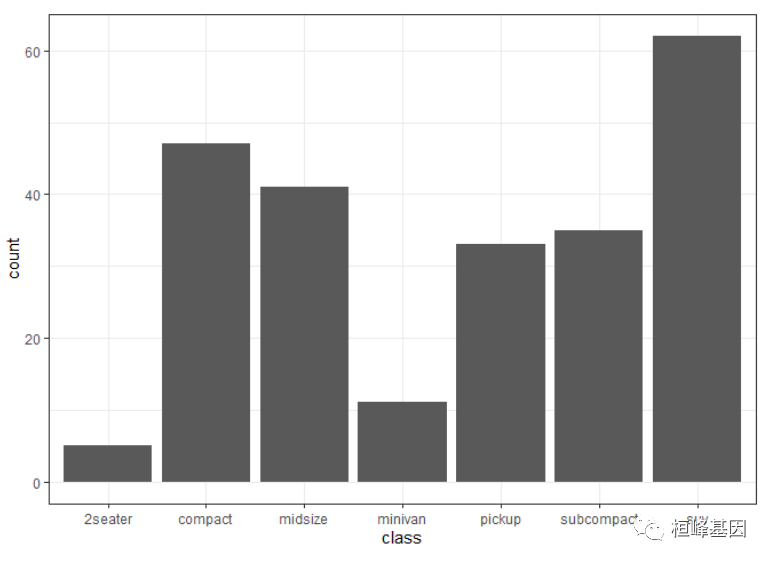
3. 简单柱状图

以每个x在数据集中出现的总数为y轴。

# geom_bar is designed to make it easy to create bar charts that show counts
# (or sums of weights)
ggplot(mpg, aes(class)) + geom_bar() + theme_bw()

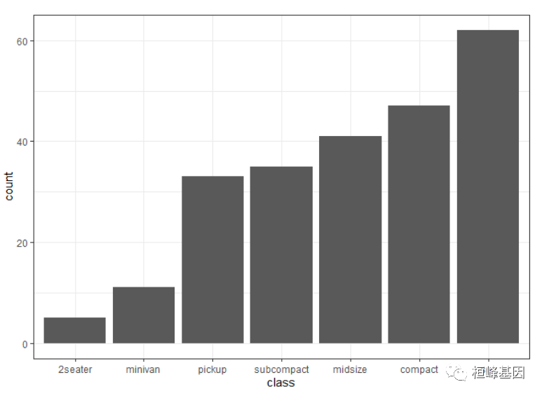
4. 简单柱状图排序

ggplot2中一般数据和视觉元素映射是分开的，如果需要对柱状图排序，就需要对数据进行排序处理。数据的处理及转换可以参考公众号FigDraw 3. SCI 文章绘图必备 R 数据转换

library(dplyr)
library(forcats)
data_sorted <- mpg %>%
    group_by(class) %>%
    summarise(count = n()) %>%
    mutate(class = fct_reorder(class, count))

ggplot() + geom_bar(data = data_sorted, aes(x = class, y = count), stat = "identity") +
    theme_bw()

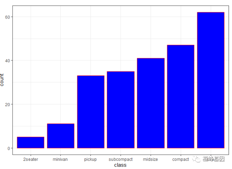
5. 外框颜色和填充颜色

参数color控制外框颜色，fill控制填充颜色。

ggplot() + geom_bar(data = data_sorted, aes(x = class, y = count), stat = "identity",
    fill = "blue", colour = "red")+theme_bw()

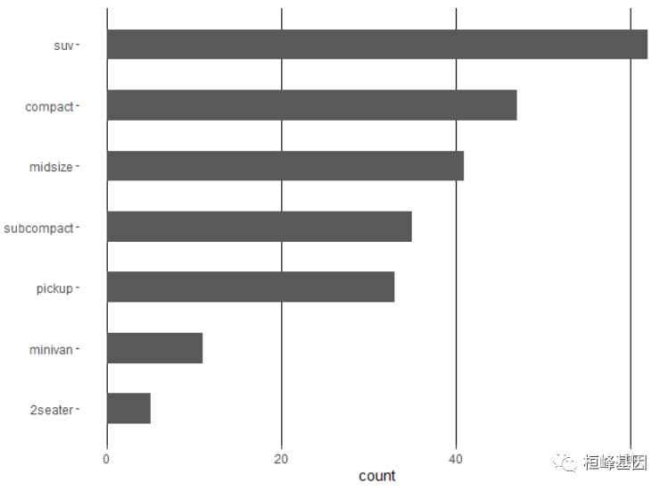
6. 水平柱状图

当数据分组标签名字过长时，有一种方法是将label旋转，这样它们就不会互相重叠。

ggplot() + geom_bar(data = data_sorted, aes(x = class, y = count), stat = "identity",
    width = 0.5, position = position_dodge(width = 0.9)) + theme(panel.grid.major.x = element_line(colour = "black"),
    panel.background = element_blank(), axis.line.y = element_blank(), axis.title.y = element_blank()) +
    coord_flip()

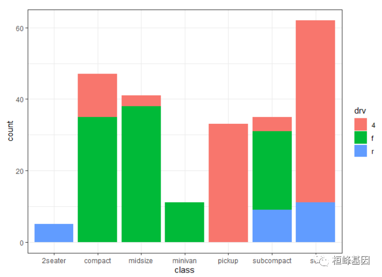
7.堆叠柱状图

分组作图的默认position 是 position = “stack”，fill参数表示将数据映射为填充颜色，color参数表示将数据映射为外框颜色。

ggplot() + geom_bar(data = mpg, aes(x = class, fill = drv), stat = "count") + theme_bw()

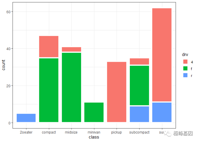
利用lwd参数增加外框线宽度，然后将外框线颜色和背景色统一，就可以形成堆叠间有间隔的柱状图。

ggplot() + geom_bar(data = mpg, aes(x = class, group = drv, fill = drv), stat = "count",
    lwd = 1.5, colour = "white") + theme_classic() + theme_bw()

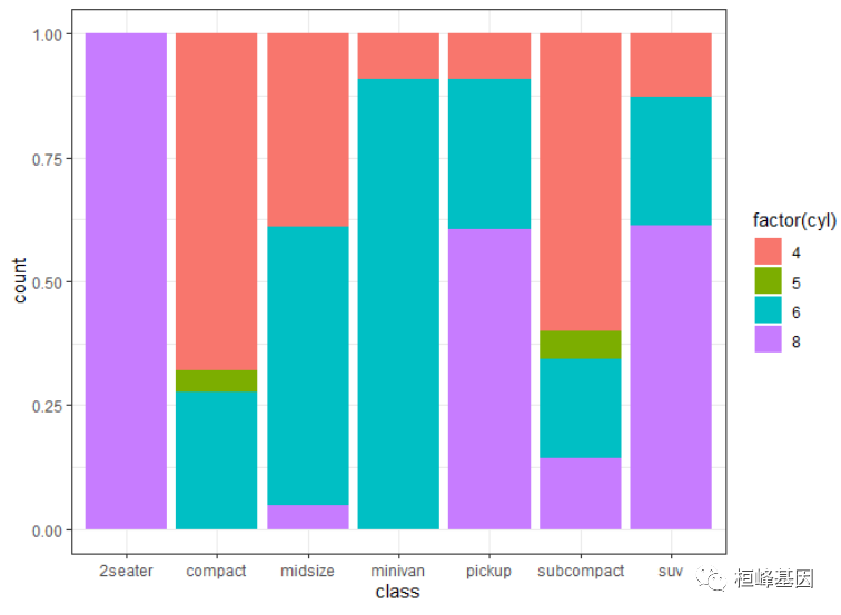
8. 百分比堆叠图

比较各组中每个类别出现次数在该组中占的百分比

ggplot() + geom_bar(data = mpg, aes(x = class, fill = factor(cyl)), position = "fill") +
    theme_bw()

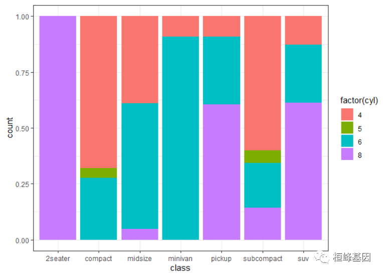
比较各组中每个类别实际值在该组中占的百分比。由于数据集data中的count就是数据集mpg中每个组别的出现次数，因此图片是一样的。

data <- mpg %>%
    group_by(class, cyl) %>%
    summarise(count = n())
ggplot() + geom_bar(data = data, aes(x = class, y = count, fill = factor(cyl)), stat = "identity",
    position = "fill") + theme_bw()

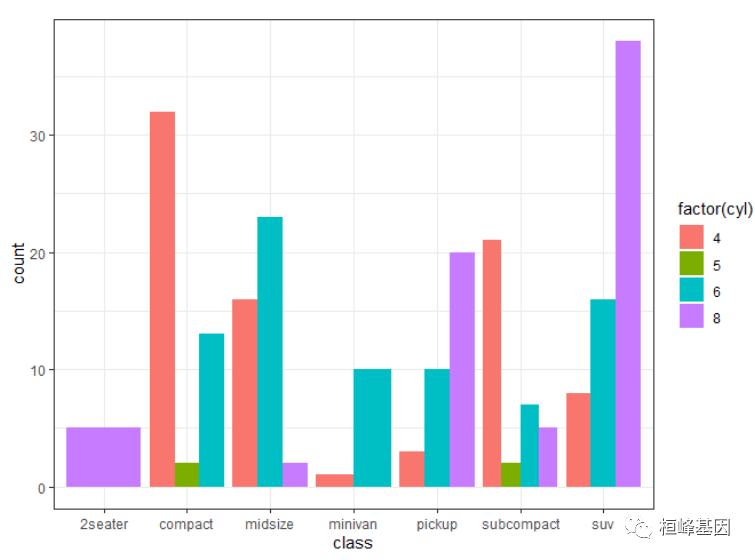
9. 并排柱状图

在aes()内部的width控制柱子的宽度，position = position_dodge()中的width控制的是一组中各柱子的间隔宽度。

ggplot() + geom_bar(data = mpg, aes(x = class, fill = factor(cyl)), position = "dodge") +
    theme_bw()

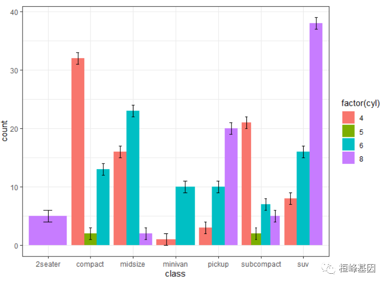
10. 添加误差线

并排的柱状图误差线和单个的相同，但需要注意一些参数。用position_dodge() 产生的并排柱状图，需要给误差线一个分组依据，然后进行的potion调试。

data <- mpg %>%
    group_by(class, cyl) %>%
    summarise(count = n())
ggplot() + geom_col(data = data, aes(x = class, y = count, fill = factor(cyl)), position = position_dodge()) +
    geom_errorbar(data = data, aes(x = class, ymin = count - 1, ymax = count + 1,
        group = factor(cyl)), width = 0.2, position = position_dodge(0.9)) + theme_bw()

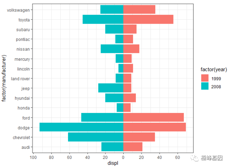
11. 金字塔图

金字塔图的核心就是找到需要分开的变量，然后以它为依据对数据进行正和负变换，然后将正负坐标轴强制设置成对应的正值。

mpg$displ <- ifelse(mpg$year == "1999", mpg$displ, -mpg$displ)

ggplot(data = mpg) + geom_col(aes(x = factor(manufacturer), y = displ, fill = factor(year))) +
    scale_y_continuous(breaks = seq(from = -100, to = 100, by = 20), labels = c(seq(100,
        0, -20), seq(20, 100, 20))) + coord_flip() + theme_bw()

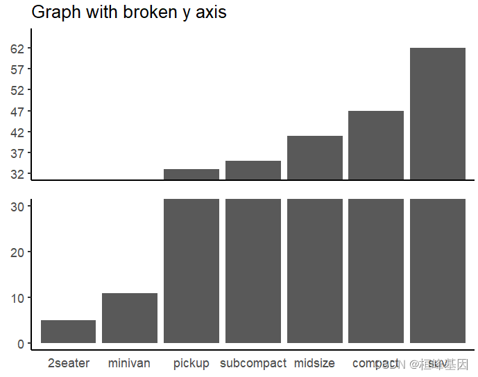
12. 坐标轴中断

当柱状图非常高，展示时可以选择截断坐标轴，形成只有底部和上部的中断柱状图。创建y轴截断的plot，如下：

require(patchwork)

theme_1 <-  theme(axis.ticks.x = element_blank(),
                  axis.title = element_blank(),
                  panel.background = element_blank(),
                  axis.line = element_line(colour = "black"))

theme_2 <-  theme(axis.text.x = element_blank(),
                  axis.ticks.x = element_blank(),
                  axis.title = element_blank(),
                  panel.background = element_blank(),
                  axis.line = element_line(colour = "black"))

p1 <- ggplot(data = data_sorted, aes(x = class, y = count)) + 
  geom_bar(stat = "identity", position = "stack") +
  coord_cartesian(ylim = c(0,30)) + theme_1
  #设置下面一半


p2 <- ggplot(data = data_sorted, aes(x = class, y = count)) + 
  geom_bar(stat = "identity", position = "stack") +
  coord_cartesian(ylim = c(32,65)) + 
  scale_y_continuous(breaks = # 按值设置breaks
                       seq(from = 32, to = 65, by = 5)) +
  labs( title = "Broken y axis")+
  theme_2

p2 /p1