


单细胞生信分析教程并配有视频在线教程,目前整理出来的相关教程目录如下:
SCS【4】单细胞转录组数据可视化分析 (Seurat 4.0)
SCS【6】单细胞转录组之细胞类型自动注释 (SingleR)
SCS【7】单细胞转录组之轨迹分析 (Monocle 3) 聚类、分类和计数细胞
SCS【8】单细胞转录组之筛选标记基因 (Monocle 3)
SCS【9】单细胞转录组之构建细胞轨迹 (Monocle 3)
SCS【10】单细胞转录组之差异表达分析 (Monocle 3)
SCS【11】单细胞ATAC-seq 可视化分析 (Cicero)
SCS【12】单细胞转录组之评估不同单细胞亚群的分化潜能 (Cytotrace)
SCS【13】单细胞转录组之识别细胞对“基因集”的响应 (AUCell)
SCS【15】细胞交互:受体-配体及其相互作用的细胞通讯数据库 (CellPhoneDB)
SCS【16】从肿瘤单细胞RNA-Seq数据中推断拷贝数变化 (inferCNV)
SCS【17】从单细胞转录组推断肿瘤的CNV和亚克隆 (copyKAT)
SCS【18】细胞交互:受体-配体及其相互作用的细胞通讯数据库 (iTALK)
简介
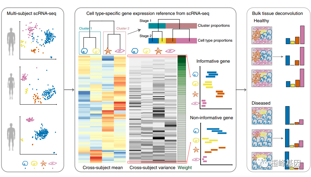
疾病相关组织中细胞类型组成的认识是确定疾病细胞靶标的重要一步。我们提出了 MuSiC,一种利用单细胞 RNA 测序 (RNA-seq) 数据中的细胞类型特异性基因表达来描述复杂组织中大量RNA-seq数据中的细胞类型组成的方法。通过对显示跨学科和跨细胞一致性的基因进行适当加权,MuSiC 能够将细胞类型特定的基因表达信息从一个数据集转移到另一个数据集。当应用于人、小鼠和大鼠的胰岛和全肾表达数据时,MuSiC 优于现有的方法,特别是对于具有密切相关细胞类型的组织。MuSiC能够表征复杂组织的细胞异质性,以了解疾病机制。由于大量组织数据比单细胞 RNA-seq 更容易获得,MuSiC 允许利用大量与疾病相关的大量组织 RNA-seq 数据来阐明细胞类型在疾病中的贡献。
软件包安装
# install devtools if necessary
install.packages('devtools')
if (!require("BiocManager", quietly = TRUE))
  install.packages("BiocManager")

BiocManager::install("TOAST")
# install the MuSiC package
devtools::install_github('xuranw/MuSiC')
数据读取
MuSiC使用两种类型的输入数据:
从RNA测序中获得的Bulk表达,这是各种细胞类型的混合表达,数据主要是 RPKM和TPM;
通过单细胞RNA测序(scRNA-seq)获得多主体单细胞表达。scRNA-seq的细胞类型是预先确定的。这些可作为估计大量数据的单元类型比例的参考。
MuSiC要求Bulk和单细胞表达的原始读取计数。
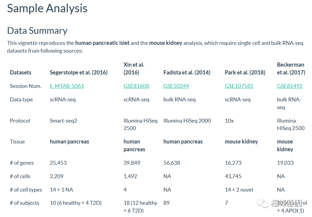
例子再现了人类胰岛和小鼠肾脏的分析,这需要来自以下来源的单细胞和Bulk RNA-seq数据集,数据下载:
https://xuranw.github.io/MuSiC/articles/pages/data.html
人体胰腺的bulk转录组数据
Fadista等人(2014)的数据集包含来自人类胰岛批量RNA-seq的原始读取计数数据,用于研究健康和高低血糖条件下的葡萄糖代谢。对于本文的目的,数据集是经过预处理的,除了read counts,该数据集还包含每个受试者的糖化血红蛋白水平、BMI、性别和年龄信息。
library(MuSiC)
library(Biobase)
GSE50244.bulk.eset = readRDS("data/GSE50244bulkeset.rds")
GSE50244.bulk.eset
## ExpressionSet (storageMode: lockedEnvironment)
## assayData: 32581 features, 89 samples
##   element names: exprs
## protocolData: none
## phenoData
##   sampleNames: Sub1 Sub2 ... Sub89 (89 total)
##   varLabels: sampleID SubjectName ... tissue (7 total)
##   varMetadata: labelDescription
## featureData: none
## experimentData: use 'experimentData(object)'
## Annotation:
bulk.mtx = exprs(GSE50244.bulk.eset)
bulk.meta = exprs(GSE50244.bulk.eset)
人胰腺单细胞数据
单细胞数据来自Segerstolpe等人(2016),该数据限制了2209个细胞中25453个基因的读取计数。这里我们只包括来自6个健康受试者的1097个细胞以SingleCellExperiment的形式获得。
EMTAB.sce = readRDS("data/EMTABsce_healthy.rds")
EMTAB.sce
## class: SingleCellExperiment
## dim: 25453 1097
## metadata(0):
## assays(1): counts
## rownames(25453): SGIP1 AZIN2 ... KIR2DL2 KIR2DS3
## rowData names(1): gene.name
## colnames(1097): AZ_A10 AZ_A11 ... HP1509101_P8 HP1509101_P9
## colData names(4): sampleID SubjectName cellTypeID cellType
## reducedDimNames(0):
## mainExpName: NULL
## altExpNames(0):
另一个单细胞数据来自Xin et al.(2016),有39849个基因和1492个细胞以ExpressionSet的形式获得。
XinT2D.sce = readRDS("data/XinT2Dsce.rds")
XinT2D.sce
## class: SingleCellExperiment
## dim: 39849 1492
## metadata(0):
## assays(1): counts
## rownames(39849): A1BG A2M ... LOC102724004 LOC102724238
## rowData names(1): gene.name
## colnames(1492): Sample_1 Sample_2 ... Sample_1491 Sample_1492
## colData names(5): sampleID SubjectName cellTypeID cellType Disease
## reducedDimNames(0):
## mainExpName: NULL
## altExpNames(0):
实操
MuSiC不选择标记基因,而是给每个基因赋予权重。加权方案基于跨学科变异:上加权基因低变异,下加权基因高变异。在这里,我们用人类胰腺数据集一步一步地演示。
Bulk 组织细胞类型估计
对Fadista等人(2014)的89例受试者进行反褶积,使用bulk数据GSE50244.bulk.eset和单细胞reference EMTAB.eset。估计限制在6种主要细胞类型:α、β、δ、γ、腺泡和导管,占整个胰岛的90%以上。细胞类型比例由函数music_prop估计。
在所包含的细胞类型中,估计的比例被归一化,总和为1。这里我们使用GSE50244.bulk.eset作为bulk.eset输入,EMTAB.eset作为sc.sce输入。集群被指定为cellType,而samples被指定为sampleID。如前所述,我们只包括6种主要的细胞类型作为select.ct。
# Estimate cell type proportions
Est.prop.GSE50244 = music_prop(bulk.mtx = bulk.mtx, sc.sce = EMTAB.sce, clusters = "cellType",
    samples = "sampleID", select.ct = c("alpha", "beta", "delta", "gamma", "acinar",
        "ductal"), verbose = F)
names(Est.prop.GSE50244)
## [1] "Est.prop.weighted" "Est.prop.allgene"  "Weight.gene"
## [4] "r.squared.full"    "Var.prop"

# Jitter plot of estimated cell type proportions
jitter.fig = Jitter_Est(list(data.matrix(Est.prop.GSE50244$Est.prop.weighted), data.matrix(Est.prop.GSE50244$Est.prop.allgene)),
    method.name = c("MuSiC", "NNLS"), title = "Jitter plot of Est Proportions")

# A more sophisticated jitter plot is provided as below. We seperated the T2D
# subjects and normal subjects by their HbA1c levels.
library(reshape2)
m.prop.GSE50244 = rbind(melt(Est.prop.GSE50244$Est.prop.weighted), melt(Est.prop.GSE50244$Est.prop.allgene))

colnames(m.prop.GSE50244) = c("Sub", "CellType", "Prop")
m.prop.GSE50244$CellType = factor(m.prop.GSE50244$CellType, levels = c("alpha", "beta",
    "delta", "gamma", "acinar", "ductal"))
m.prop.GSE50244$Method = factor(rep(c("MuSiC", "NNLS"), each = 89 * 6), levels = c("MuSiC",
    "NNLS"))
m.prop.GSE50244$HbA1c = rep(GSE50244.bulk.eset$hba1c, 2 * 6)
m.prop.GSE50244 = m.prop.GSE50244[!is.na(m.prop.GSE50244$HbA1c), ]
m.prop.GSE50244$Disease = factor(c("Normal", "T2D")[(m.prop.GSE50244$HbA1c > 6.5) +
    1], levels = c("Normal", "T2D"))
m.prop.GSE50244$D = (m.prop.GSE50244$Disease == "T2D")/5
m.prop.GSE50244 = rbind(subset(m.prop.GSE50244, Disease == "Normal"), subset(m.prop.GSE50244,
    Disease != "Normal"))

jitter.new = ggplot(m.prop.GSE50244, aes(Method, Prop)) + geom_point(aes(fill = Method,
    color = Disease, stroke = D, shape = Disease), size = 2, alpha = 0.7, position = position_jitter(width = 0.25,
    height = 0)) + facet_wrap(~CellType, scales = "free") + scale_colour_manual(values = c("white",
    "gray20")) + scale_shape_manual(values = c(21, 24)) + theme_minimal()

library(cowplot)
plot_grid(jitter.fig, jitter.new, labels = "auto")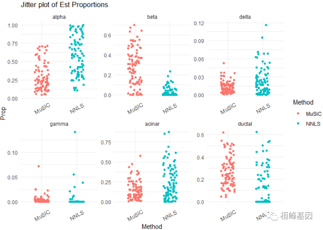
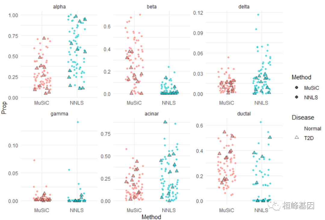
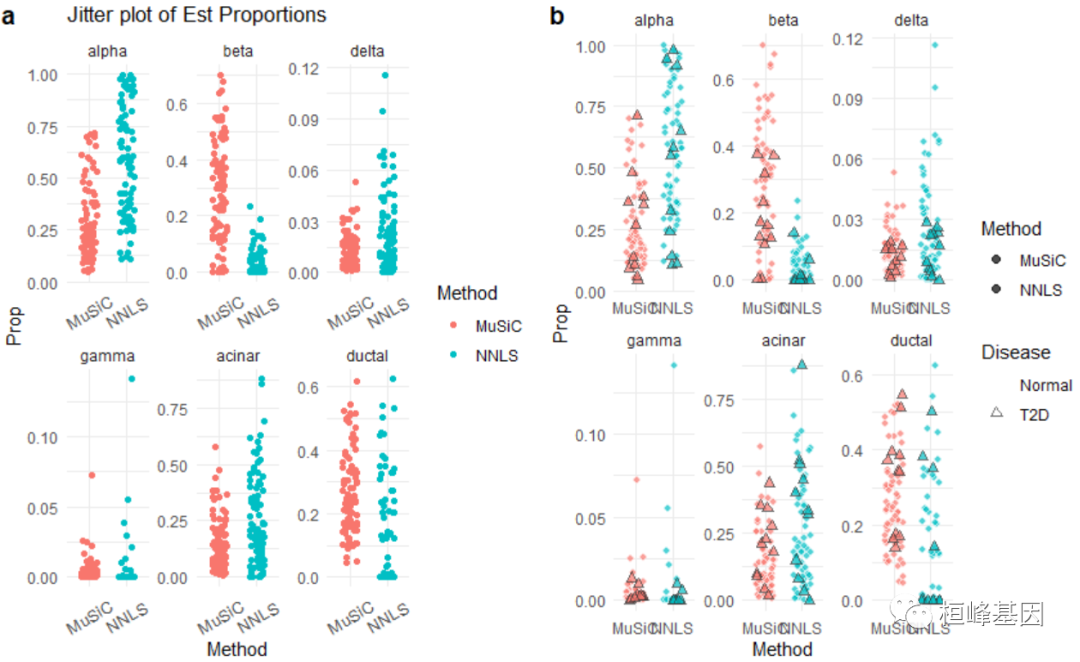
众所周知,β细胞比例与T2D疾病状态相关。在T2D进展过程中,β细胞数量减少。T2D最重要的检查之一是HbA1c(血红蛋白A1c)检查。当HbA1c水平大于6.5%时,诊断为T2D。让我们看看β细胞比例与糖化血红蛋白水平。
# Create dataframe for beta cell proportions and HbA1c levels
m.prop.ana = data.frame(pData(GSE50244.bulk.eset)[rep(1:89, 2), c("age", "bmi", "hba1c",
    "gender")], ct.prop = c(Est.prop.GSE50244$Est.prop.weighted[, 2], Est.prop.GSE50244$Est.prop.allgene[,
    2]), Method = factor(rep(c("MuSiC", "NNLS"), each = 89), levels = c("MuSiC",
    "NNLS")))
colnames(m.prop.ana)[1:4] = c("Age", "BMI", "HbA1c", "Gender")
m.prop.ana = subset(m.prop.ana, !is.na(HbA1c))
m.prop.ana$Disease = factor(c("Normal", "T2D")[(m.prop.ana$HbA1c > 6.5) + 1], c("Normal",
    "T2D"))
m.prop.ana$D = (m.prop.ana$Disease == "T2D")/5

ggplot(m.prop.ana, aes(HbA1c, ct.prop)) + geom_smooth(method = "lm", se = FALSE,
    col = "black", lwd = 0.25) + geom_point(aes(fill = Method, color = Disease, stroke = D,
    shape = Disease), size = 2, alpha = 0.7) + facet_wrap(~Method) + ggtitle("HbA1c vs Beta Cell Type Proportion") +
    theme_minimal() + scale_colour_manual(values = c("white", "gray20")) + scale_shape_manual(values = c(21,
    24))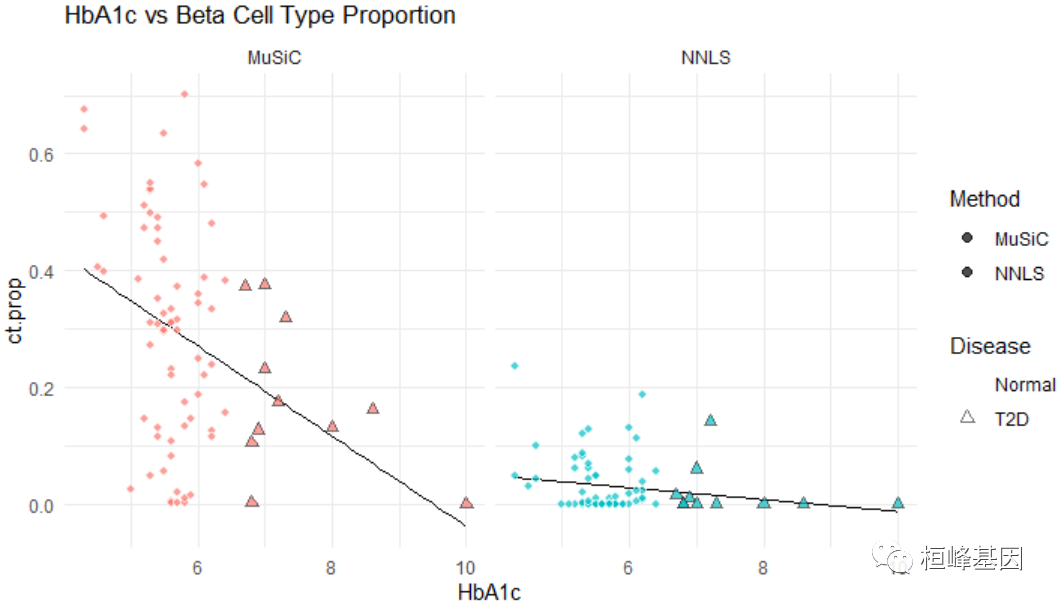
通过线性回归得到数值评价。调整年龄、BMI和性别后,HbA1c水平与β细胞比例呈显著负相关。
lm.beta.MuSiC = lm(ct.prop ~ HbA1c + Age + BMI + Gender, data = subset(m.prop.ana,
    Method == "MuSiC"))
lm.beta.NNLS = lm(ct.prop ~ HbA1c + Age + BMI + Gender, data = subset(m.prop.ana,
    Method == "NNLS"))
summary(lm.beta.MuSiC)
##
## Call:
## lm(formula = ct.prop ~ HbA1c + Age + BMI + Gender, data = subset(m.prop.ana,
##     Method == "MuSiC"))
##
## Residuals:
##      Min       1Q   Median       3Q      Max
## -0.27768 -0.13186 -0.01096  0.10661  0.35790
##
## Coefficients:
##               Estimate Std. Error t value Pr(>|t|)
## (Intercept)   0.877022   0.190276   4.609 1.71e-05 ***
## HbA1c        -0.061396   0.025403  -2.417   0.0182 *
## Age           0.002639   0.001772   1.489   0.1409
## BMI          -0.013620   0.007276  -1.872   0.0653 .
## GenderFemale -0.079874   0.039274  -2.034   0.0457 *
## ---
## Signif. codes:  0 '***' 0.001 '**' 0.01 '*' 0.05 '.' 0.1 ' ' 1
##
## Residual standard error: 0.167 on 72 degrees of freedom
## Multiple R-squared:  0.2439,	Adjusted R-squared:  0.2019
## F-statistic: 5.806 on 4 and 72 DF,  p-value: 0.0004166
summary(lm.beta.NNLS)
##
## Call:
## lm(formula = ct.prop ~ HbA1c + Age + BMI + Gender, data = subset(m.prop.ana,
##     Method == "NNLS"))
##
## Residuals:
##      Min       1Q   Median       3Q      Max
## -0.04671 -0.02918 -0.01795  0.01394  0.19362
##
## Coefficients:
##                Estimate Std. Error t value Pr(>|t|)
## (Intercept)   0.0950960  0.0546717   1.739   0.0862 .
## HbA1c        -0.0093214  0.0072991  -1.277   0.2057
## Age           0.0005268  0.0005093   1.035   0.3044
## BMI          -0.0015116  0.0020906  -0.723   0.4720
## GenderFemale -0.0037650  0.0112844  -0.334   0.7396
## ---
## Signif. codes:  0 '***' 0.001 '**' 0.01 '*' 0.05 '.' 0.1 ' ' 1
##
## Residual standard error: 0.04799 on 72 degrees of freedom
## Multiple R-squared:  0.0574,	Adjusted R-squared:  0.005028
## F-statistic: 1.096 on 4 and 72 DF,  p-value: 0.3651
细胞类型预分组的细胞类型比例估计
实体瘤组织通常包含密切相关的细胞类型,这些细胞类型之间的基因表达相关性导致共线性,使得难以在bulk数据中解析它们的相对比例。为了处理共线性,MuSiC采用了一种树引导的过程,递归地放大密切相关的细胞类型。简单地说,我们首先将相似的细胞类型分组到相同的cluster中,并估计cluster的比例,然后在每个cluster中递归地重复这个过程。在每个递归阶段,我们只使用cluster内方差低的基因,即跨细胞一致性基因。这是至关重要的,因为高方差异基因的平均表达估计受到scRNA-seq实验中细胞捕获的普遍偏差的影响,因此不能作为可靠的参考。
数据准备
bulk数据来时GEO(GSE81492)(见Beckerman et al. 2017)包含原始RNA-seq和示例注释数据。
单细胞数据来自GEO数据库(GSE107585)(见Park et al. 2018),该数据集有43745个细胞中16273个基因的 read counts。
Mouse.bulk.eset = readRDS("data/Mousebulkeset.rds")
Mouse.bulk.eset
## ExpressionSet (storageMode: lockedEnvironment)
## assayData: 19033 features, 10 samples
##   element names: exprs
## protocolData: none
## phenoData
##   sampleNames: control.NA.27 control.NA.30 ... APOL1.GNA78M (10 total)
##   varLabels: sampleID SubjectName Control
##   varMetadata: labelDescription
## featureData: none
## experimentData: use 'experimentData(object)'
## Annotation:

Mousesub.sce = readRDS("data/Mousesub_sce.rds")
Mousesub.sce
## class: SingleCellExperiment
## dim: 16273 10000
## metadata(0):
## assays(1): counts
## rownames(16273): Rp1 Sox17 ... DHRSX CAAA01147332.1
## rowData names(0):
## colnames(10000): TGGTTCCGTCGGCTCA-2 CGAGCCAAGCGTCAAG-4 ...
##   GTATTCTGTAGCTAAA-2 GAGCAGAGTCAACATC-1
## colData names(4): sampleID SubjectName cellTypeID cellType
## reducedDimNames(0):
## mainExpName: NULL
## altExpNames(0):
levels(Mousesub.sce$cellType)
##  [1] "Endo"     "Podo"     "PT"       "LOH"      "DCT"      "CD-PC"
##  [7] "CD-IC"    "CD-Trans" "Novel1"   "Fib"      "Macro"    "Neutro"
## [13] "B lymph"  "T lymph"  "NK"       "Novel2"
聚类单细胞数据
在之前的MuSiC估计过程中,第一步是从单细胞参考中生成设计矩阵、相对丰度的跨学科平均值、相对丰度的跨学科方差和平均值大小。由函数music_basis来计算。
# Produce the first step information
Mousesub.basis = music_basis(Mousesub.sce, clusters = "cellType", samples = "sampleID",
    select.ct = c("Endo", "Podo", "PT", "LOH", "DCT", "CD-PC", "CD-IC", "Fib", "Macro",
        "Neutro", "B lymph", "T lymph", "NK"))

# Plot the dendrogram of design matrix and cross-subject mean of realtive
# abundance
par(mfrow = c(1, 2))
d <- dist(t(log(Mousesub.basis$Disgn.mtx + 1e-06)), method = "euclidean")
# Hierarchical clustering using Complete Linkage
hc1 <- hclust(d, method = "complete")
# Plot the obtained dendrogram
plot(hc1, cex = 0.6, hang = -1, main = "Cluster log(Design Matrix)")
d <- dist(t(log(Mousesub.basis$M.theta + 1e-08)), method = "euclidean")
# Hierarchical clustering using Complete Linkage hc2 <- hclust(d, method =
# 'complete' )
hc2 <- hclust(d, method = "complete")
# Plot the obtained dendrogram
plot(hc2, cex = 0.6, hang = -1, main = "Cluster log(Mean of RA)")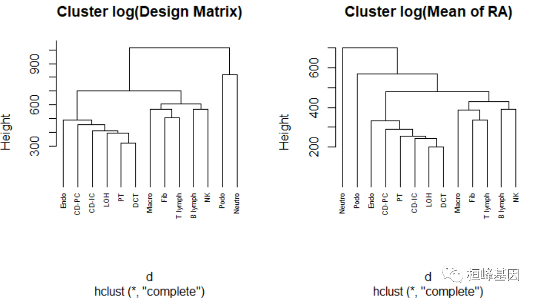
基于细胞类型预分组的大块组织细胞类型估计
我们手动指定cluster并使用cluster信息注释单细胞。
clusters.type = list(C1 = "Neutro", C2 = "Podo", C3 = c("Endo", "CD-PC", "LOH", "CD-IC",
    "DCT", "PT"), C4 = c("Macro", "Fib", "B lymph", "NK", "T lymph"))

cl.type = as.character(Mousesub.sce$cellType)

for (cl in 1:length(clusters.type)) {
    cl.type[cl.type %in% clusters.type[[cl]]] = names(clusters.type)[cl]
}
Mousesub.sce$clusterType = factor(cl.type, levels = c(names(clusters.type), "CD-Trans",
    "Novel1", "Novel2"))

# 13 selected cell types
s.mouse = unlist(clusters.type)
s.mouse
##        C1        C2       C31       C32       C33       C34       C35       C36
##  "Neutro"    "Podo"    "Endo"   "CD-PC"     "LOH"   "CD-IC"     "DCT"      "PT"
##       C41       C42       C43       C44       C45
##   "Macro"     "Fib" "B lymph"      "NK" "T lymph"
然后,我们选择了C3(上皮细胞)和C4(免疫细胞)集群中差异表达的基因,music_prop函数。聚类用于预聚类估计细胞类型。基本输入与music_prop相同,除了两个唯一的输入:groups和group.markers。groups传递了表型数据中更高集群的列名。cluster内差异表达基因通过group.marker传递。
load("data/IEmarkers.RData")
# This RData file provides two vectors of gene names Epith.marker and
# Immune.marker

# We now construct the list of group marker
IEmarkers = list(NULL, NULL, Epith.marker, Immune.marker)
names(IEmarkers) = c("C1", "C2", "C3", "C4")
# The name of group markers should be the same as the cluster names

Est.mouse.bulk = music_prop.cluster(bulk.mtx = exprs(Mouse.bulk.eset), sc.sce = Mousesub.sce,
    group.markers = IEmarkers, clusters = "cellType", groups = "clusterType", samples = "sampleID",
    clusters.type = clusters.type)
基准评价
基准数据集由XinT2D.eset的单细胞数据累加而成。通过函数bulk_construct构造人工批量数据。输入是单个单元数据集、聚类名称(clusters)、样本名称(samples)和选定的细胞类型(select.ct)。bulk_construct返回一个人工bulk的ExpressionSet。计数,实际细胞类型的矩阵计数为num.real。
XinT2D.construct.full = bulk_construct(XinT2D.sce, clusters = "cellType", samples = "SubjectName")

names(XinT2D.construct.full)
## [1] "bulk.counts" "num.real"

dim(XinT2D.construct.full$bulk.counts)
## [1] 39849    18

XinT2D.construct.full$bulk.counts[1:5, 1:5]
##       Non T2D 1 Non T2D 2 Non T2D 3 Non T2D 5 Non T2D 6
## A1BG        297       269       127      1042       262
## A2M           1         1        19        21         2
## A2MP1       493         0         0         0         0
## NAT1       1856        36       278       559      1231
## NAT2          1         0         0         0         0

head(XinT2D.construct.full$num.real)
##           beta alpha delta gamma
## Non T2D 1   13    53     5     3
## Non T2D 2   13     4     2     5
## Non T2D 3   10    27     3     2
## Non T2D 5   22    23     5     2
## Non T2D 6    7    36     4     1
## Non T2D 7   15     8     0     4
细胞类型比例的估计:
# calculate cell type proportions
XinT2D.construct.full$prop.real = relative.ab(XinT2D.construct.full$num.real, by.col = FALSE)
head(XinT2D.construct.full$prop.real)
## beta alpha delta gamma
## Non T2D 1 0.1756757 0.7162162 0.06756757 0.04054054
## Non T2D 2 0.5416667 0.1666667 0.08333333 0.20833333
## Non T2D 3 0.2380952 0.6428571 0.07142857 0.04761905
## Non T2D 5 0.4230769 0.4423077 0.09615385 0.03846154
## Non T2D 6 0.1458333 0.7500000 0.08333333 0.02083333
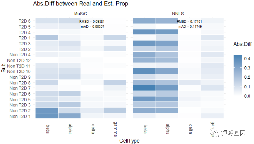
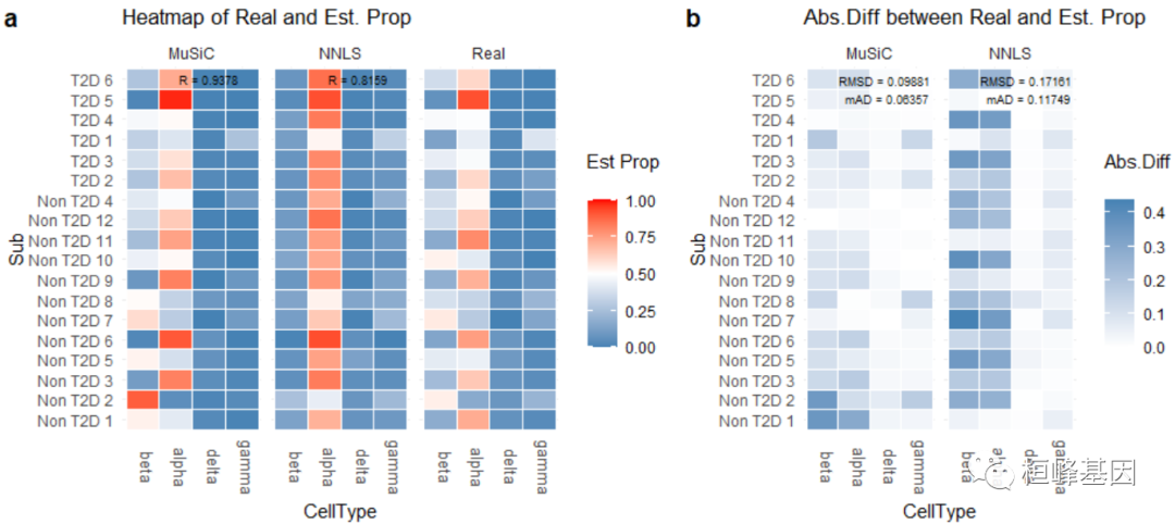
## Non T2D 7 0.5555556 0.2962963 0.00000000 0.14814815数值评估由Eval_multi进行,它比较真实和估计的细胞类型比例 包括:
均方根偏差(RMSD);
平均绝对差(mAD);
皮尔逊相关系数(R)。
细胞类型比例的可视化由Prop_comp_multi, Abs_diff_multi和Scatter_multi函数:
# Estimate cell type proportions of artificial bulk data
Est.prop.Xin = music_prop(bulk.mtx = XinT2D.construct.full$bulk.counts, sc.sce = EMTAB.sce,
    clusters = "cellType", samples = "sampleID", select.ct = c("alpha", "beta", "delta",
        "gamma"))

# Estimation evaluation

Eval_multi(prop.real = data.matrix(XinT2D.construct.full$prop.real), prop.est = list(data.matrix(Est.prop.Xin$Est.prop.weighted),
    data.matrix(Est.prop.Xin$Est.prop.allgene)), method.name = c("MuSiC", "NNLS"))
##          RMSD     mAD      R
## MuSiC 0.09881 0.06357 0.9378
## NNLS  0.17161 0.11749 0.8159


library(cowplot)
prop.comp.fig = Prop_comp_multi(prop.real = data.matrix(XinT2D.construct.full$prop.real),
    prop.est = list(data.matrix(Est.prop.Xin$Est.prop.weighted), data.matrix(Est.prop.Xin$Est.prop.allgene)),
    method.name = c("MuSiC", "NNLS"), title = "Heatmap of Real and Est. Prop")

abs.diff.fig = Abs_diff_multi(prop.real = data.matrix(XinT2D.construct.full$prop.real),
    prop.est = list(data.matrix(Est.prop.Xin$Est.prop.weighted), data.matrix(Est.prop.Xin$Est.prop.allgene)),
    method.name = c("MuSiC", "NNLS"), title = "Abs.Diff between Real and Est. Prop")

plot_grid(prop.comp.fig, abs.diff.fig, labels = "auto", rel_widths = c(4, 3))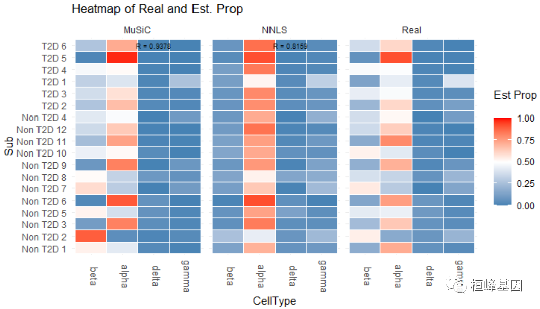
Reference:
Wang, X., Park, J., Susztak, K. et al. Bulk tissue cell type deconvolution with multi-subject single-cell expression reference. Nat Commun 10, 380 (2019).
Baron, Maayan, Adrian Veres, Samuel L Wolock, Aubrey L Faust, Renaud Gaujoux, Amedeo Vetere, Jennifer Hyoje Ryu, et al. 2016. “A Single-Cell Transcriptomic Map of the Human and Mouse Pancreas Reveals Inter-and Intra-Cell Population Structure.” Cell Systems 3 (4): 346–60.
Beckerman, Pazit, Jing Bi-Karchin, Ae Seo Deok Park, Chengxiang Qiu, Patrick D Dummer, Irfana Soomro, Carine M Boustany-Kari, et al. 2017. “Transgenic Expression of Human Apol1 Risk Variants in Podocytes Induces Kidney Disease in Mice.” Nature Medicine 23 (4): 429.
Fadista, João, Petter Vikman, Emilia Ottosson Laakso, Inês Guerra Mollet, Jonathan Lou Esguerra, Jalal Taneera, Petter Storm, et al. 2014. “Global Genomic and Transcriptomic Analysis of Human Pancreatic Islets Reveals Novel Genes Influencing Glucose Metabolism.” Proceedings of the National Academy of Sciences 111 (38): 13924–29.
这个细胞互作软件包代码量还是很多的,需要具有一定 R 语言编程基础,并不是看起来那么简单,所有好多老师想直接自己学习教程来分析,但是实质上没有基础还是很难实现,每步报错都不知道该怎样处理,是最崩溃的,所以有需求的老师可以联系桓峰基因,提供最优质的服务!!!
桓峰基因,铸造成功的您!
未来桓峰基因公众号将不间断的推出单细胞系列生信分析教程,
敬请期待!!
桓峰基因和投必得合作,文章润色优惠85折,需要文章润色的老师可以直接到网站输入领取桓峰基因专属优惠券码:KYOHOGENE,然后上传,付款时选择桓峰基因优惠券即可享受85折优惠哦!https://www.topeditsci.com/
有想进生信交流群的老师可以扫最后一个二维码加微信,备注“单位+姓名+目的”,有些想发广告的就免打扰吧,还得费力气把你踢出去!


 4781
4781

 被折叠的 条评论
为什么被折叠?
被折叠的 条评论
为什么被折叠?
 到【灌水乐园】发言


