OpenGL 4 Shading Language Cookbook chapter 2——The Basics of GLSL Shaders

introduction

shaders were first added into opengl in version 2.0, introducing programmability into the formerly 之前胡 fixed-function opengl pipeline.
shaders give us the power to implement alternative rendering algorithms and a greater degree of flexibility in the implementation of those techniques.

with shaders, we can run custom code directly on GPU, providing us with the opportunity to leverage the high degree of parallelism available with modern gpus.

shaders are implemented using the opengl shading language – glsl.
the glsl is syntactically similar to C, which should make it easier for experienced opengl programers to learn.

due to the nature of this text, i will not present a thorough introduction to glsl here.
instead, if u are new to glsl, reading through these recipes should help u to learn the language by example.
if u are already comfortable with glsl, but do not have experience with version 4.x, u will see how to implement these techniques utilizing these newer api.
however, before we jump into glsl progamming, let us take a look at how vertex and fragment shaders fit within the opengl pipeline.

vertex and fragment shaders

in opengl version 4.3, there are six shader stages/types:
vertex, geometery, tessellation control, tessellation evaluation, fragment, and compute.

in this chapter we will focus only on the vetex and fragment stages.

in chapter6, using geometry and tessellation shaders.
i will provide some recipes for working with the geometry and tessellation shaders, and in chapter 10, using compute shaders, i will focus specifically on compute shaders.

shaders replace parts of the opengl pipeline.
more specifically, they make those parts of the pipeline programmable.
the following block diagram shows a simplified view of the opengl pipeline with only the vertex and fragment shaders installed:

vertex data is sent down the pipeline and arrives at the vertex shader via shader input variables.
the vetex shader’s input variables correspond to the vertex attributes (refer to the sending data to a shader using vertex attributes and vertex buffer objects recipe in chapter 1, gettting started with glsl).

in general, a shader receives its input via programmer defined input variables, and the data for those variables comes either from the main opengl application or previous pipeline stages (other shaders).

for example, a fragment shader’s input variables might be fed from the output variables of the vetex shader.
data can also be provided to any shader stage using uniform variables (refer to the Sending data to a shader
using uniform variables recipe, in Chapter 1, Getting Started with GLSL).

these are used for information that changes less often than vertex attributes (for example, matrices, light position, and other settings).

the following figure shows a simplified view of the relationships between input and output variables when there are two shaders active (vertex and fragment):

the vertex shader is executed once for each vertex, usually in parallel. the data corresponding to the position of the vertex must be transformed into clip coordinates and assigned to the output variable gl_Position before the vertex shader finishes execution.
the vertex shader can send other information down the pipeline using shader output variables.
for example, the vertex shader might also compute the color associated with the vertex.
that color would be passed to later stages via an appropriate output variable.

Between the vertex and fragment shader, the vertices are assembled into primitives, clipping
takes place, and the viewport transformation is applied (among other operations). The rasterization process then takes place and the polygon is filled (if necessary). The fragment shader is executed once for each fragment (pixel) of the polygon being rendered (typically in
parallel). Data provided from the vertex shader is (by default) interpolated in a perspective correct manner, and provided to the fragment shader via shader input variables. The fragment shader determines the appropriate color for the pixel and sends it to the frame buffer using output variables. The depth information is handled automatically.

replicating the old fixed functionality
Programmable shaders give us tremendous power and flexibility. However, in some cases we might just want to re-implement the basic shading techniques that were used in the default fixed-function pipeline, or perhaps use them as a basis for other shading techniques. Studying the basic shading algorithm of the old fixed-function pipeline can also be a good way to get started when learning about shader programming.
In this chapter, we’ll look at the basic techniques for implementing shading similar to that of the old fixed-function pipeline. We’ll cover the standard ambient, diffuse, and specular (ADS) shading algorithm, the implementation of two-sided rendering, and flat shading. Along the way, we’ll also see some examples of other GLSL features such as functions, subroutines, and the discard keyword.

The algorithms presented within this chapter are largely unoptimized. I present them this way to avoid additional confusion for someone who is learning the techniques for the first time. We’ll look at a few optimization techniques at the end of some recipes, and some more in the next chapter.

Implementing diffuse, per-vertex shading
with a single point light source

One of the simplest shading techniques is to assume that the surface exhibits purely diffuse
reflection. That is to say that the surface is one that appears to scatter light in all directions
equally, regardless of direction. Incoming light strikes the surface and penetrates slightly
before being re-radiated in all directions. Of course, the incoming light interacts with the
surface before it is scattered, causing some wavelengths to be fully or partially absorbed
and others to be scattered. A typical example of a diffuse surface is a surface that has been
painted with a matte paint. The surface has a dull look with no shine at all.
The following screenshot shows a torus rendered with diffuse shading:

The mathematical model for diffuse reflection involves two vectors: the direction from the
surface point to the light source (s), and the normal vector at the surface point (n). The
vectors are represented in the following diagram:

The amount of incoming light (or radiance) that reaches the surface is partially dependent on the orientation of the surface with respect to the light source. The physics of the situation tells us that the amount of radiation that reaches a point on a surface is maximal when the
light arrives along the direction of the normal vector, and zero when the light is perpendicular to the normal. In between, it is proportional to the cosine of the angle between the direction towards the light source and the normal vector. So, since the dot product is proportional to the cosine of the angle between two vectors, we can express the amount of radiation striking the surface as the product of the light intensity and the dot product of s and n.

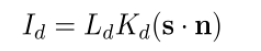
Where Ld is the intensity of the light source, and the vectors s and n are assumed to be
normalized.

As stated previously, some of the incoming light is absorbed before it is re-emitted. We can
model this interaction by using a reflection coefficient (Kd), which represents the fraction of
the incoming light that is scattered. This is sometimes referred to as the diffuse reflectivity,
or the diffuse reflection coefficient. The diffuse reflectivity becomes a scaling factor for the
incoming radiation, so the intensity of the outgoing light can be expressed as follows:
Because this model depends only on the direction towards the light source and the normal to
the surface, not on the direction towards the viewer, we have a model that represents uniform
(omnidirectional) scattering.

In this recipe, we’ll evaluate this equation at each vertex in the vertex shader and interpolate
the resulting color across the face.

Start with an OpenGL application that provides the vertex position in attribute location 0, and the vertex normal in attribute location 1 (refer to the Sending data to a shader using vertex attributes and vertex buffer objects recipe in Chapter 1, Getting Started with GLSL).
The OpenGL application also should provide the standard transformation matrices (projection, modelview, and normal) via uniform variables. The light position (in eye coordinates), Kd, and Ld should also be provided by the OpenGL application via uniform variables. Note that Kd and Ld are of type vec3. We can use vec3 to store an RGB color as well as a vector or point.

To create a shader pair that implements diffuse shading, use the following steps:

1. Use the following code for the vertex shader:

layout (location = 0) in vec3 VertexPosition;
layout (location = 1) in vec3 VertexNormal;
out vec3 LightIntensity;
uniform vec4 LightPosition;// Light position in eye coords.
uniform vec3 Kd; // Diffuse reflectivity
uniform vec3 Ld; // Light source intensity
uniform mat4 ModelViewMatrix;
uniform mat3 NormalMatrix;
uniform mat4 ProjectionMatrix;
uniform mat4 MVP; // Projection * ModelView
void main()
{
		// Convert normal and position to eye coords
		vec3 tnorm = normalize( NormalMatrix * VertexNormal);
		vec4 eyeCoords = ModelViewMatrix *
		vec4(VertexPosition,1.0));
		vec3 s = normalize(vec3(LightPosition - eyeCoords));
		// The diffuse shading equation
		LightIntensity = Ld * Kd * max( dot( s, tnorm ), 0.0 );
		// Convert position to clip coordinates and pass along
		gl_Position = MVP * vec4(VertexPosition,1.0);

2. Use the following code for the fragment shader:

in vec3 LightIntensity;
layout( location = 0 ) out vec4 FragColor;
void main() 
{
	FragColor = vec4(LightIntensity, 1.0);
}

3. Compile and link both shaders within the OpenGL application, and install the shader program prior to rendering. See Chapter 1, Getting Started with GLSL, for details about compiling, linking, and installing shaders.

The next step converts the vertex position to eye (camera) coordinates by transforming it via the model-view matrix. Then we compute the direction towards the light source by subtracting the vertex position from the light position and storing the result in s.

Next, we compute the scattered light intensity using the equation described previously and store the result in the output variable LightIntensity. Note the use of the max function here. If the dot product is less than zero, then the angle between the normal vector and the light direction is greater than 90 degrees. This means that the incoming light is coming from inside the surface.

Since such a situation is not physically possible (for a closed mesh), we use a value of 0.0. However, you may decide that you want to properly light both sides of your surface, in which case the normal vector needs to be reversed for those situations where the light is striking the back side of the surface (refer to the Implementing two-sided shading recipe in this chapter).

Finally, we convert the vertex position to clip coordinates by multiplying with the model-view projection matrix, (which is: projection * view * model) and store the result in the built-in output variable gl_Position.

注：
The subsequent stage of the OpenGL pipeline expects that the vertex position will be provided in clip coordinates in the
output variable gl_Position. This variable does not directly correspond to any input variable in the fragment shader, but is
used by the OpenGL pipeline in the primitive assembly, clipping, and rasterization stages that follow the vertex shader. It is
important that we always provide a valid value for this variable.

Since LightIntensity is an output variable from the vertex shader, its value is interpolated across the face and passed into the fragment shader. The fragment shader then simply assigns the value to the output fragment.

Diffuse shading is a technique that models only a very limited range of surfaces. It is best used for surfaces that have a “matte” appearance. 表面粗糙的 Additionally, with the technique used previously, the dark areas may look a bit too dark. In fact, those areas that are not directly illuminated are completely black. In real scenes, there is typically some light that has been reflected about the room that brightens these surfaces. In the following recipes, we’ll look at ways to model more surface types, as well as provide some light for those dark parts of the surface.

implementing per-vertex ambient, diffuse, and specular (ADS) shading

the opengl fixed function pipeline implemented a default shading technique which is very similar to the one presented here.
it models the light-surface interation as a combination of three components: ambient, diffuse, and specular.

the ambient component is intended to model light that has been reflected so many times that it appears to be emanating uniformly from all directions.
the diffuse component was discussed in the previous recipe, and represents omnidirectional reflection. 全方位
the specualr component models the shininess of the surface and represents reflection around a preferred direction.
combing these three components together can model a nice (but limited) variety of surface types.

this shading model is also sometimes called the Phong reflection modle (or Phong shading model), after Bui Tuong Phong.

an example of a torus rendered with the ADS shading model is shown in the following screenshot:

the ADS model is implemented as the sum of the three components: ambient, diffuse, and specular.
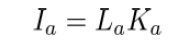
the ambient component represents light that illuminates all surfaces equally and reflects equally in all directions.
it is often used to help brighten some of the darker areas withing a scene.
since it does not depend on the incoming or outgoing directions of the light, it can be modeled simply by multiplying the light source intensity (La) by the surface reflectivity (Ka).

the diffuse component models a rough surface that scatters light in all directions (refer to
the Implementing diffuse, per-vertex shading with a single point light source recipe in this
chapter). the intensity of the outgoing light depends on the angle between the surface normal and the vector towards the light source.

The specular component is used for modeling the shininess of a surface. When a surface has
a glossy shine to it, the light is reflected off of the surface in a mirror-like fashion. The reflected
light is strongest in the direction of perfect (mirror-like) reflection. The physics of the situation
tells us that for perfect reflection, the angle of incidence 入射角 is the same as the angle of reflection
and that the vectors are coplanar 共平面 with the surface normal, as shown in the following diagram:

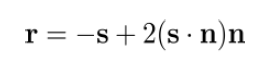
In the preceding 上图 diagram, r represents the vector of pure-reflection corresponding to the
incoming light vector (-s), and n is the surface normal. We can compute r by using the
following equation:

To model specular reflection, we need to compute the following (normalized) vectors: the
direction towards the light source (s), the vector of perfect reflection ®, the vector towards the
viewer (v), and the surface normal (n). These vectors are represented in the following diagram:

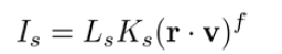
We would like the reflection to be maximal when the viewer is aligned with the vector r, and to
fall off quickly as the viewer moves further away from alignment with r. This can be modeled
using the cosine of the angle between v and r raised to some power (f).

V为视角、r为反射光线，两个之间的夹角越小，反射越强。

(Recall that the dot product is proportional to the cosine of the angle between the vectors
involved.) The larger the power, the faster the value drops towards zero as the angle between
v and r increases. Again, similar to the other components, we also introduce a specular light
intensity term (Ls) and reflectivity term (Ks).

the specular component creates specular highlights (bright spots) that are typical of glossy surfaces. 光滑的表面。

the larger the power of f in the equation, the smaller the specular highlight and the shinier the surface appears.
the value of f is typically chosen to be somewhere between 1 and 200.

putting all of this together, we have the following shading equation:

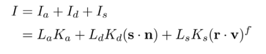
for more details about how this shading model was implemented in the fixed function pipeline, take a look at Chapter 5, Image Processing and Screen Space Techniques.

In the following code, we’ll evaluate this equation in the vertex shader, and interpolate the
color across the polygon.

In the OpenGL application, provide the vertex position in location 0 and the vertex
normal in location 1. The light position and the other configurable terms for our lighting
equation are uniform variables in the vertex shader and their values must be set from the
OpenGL application.
To create a shader pair that implements ADS shading, use the following steps:

1. Use the following code for the vertex shader:

layout (location = 0) in vec3 VertexPosition;
layout (location = 1) in vec3 VertexNormal;
out vec3 LightIntensity;
struct LightInfo 
{
	vec4 Position; // Light position in eye coords.
	vec3 La; // Ambient light intensity
	vec3 Ld; // Diffuse light intensity
	vec3 Ls; // Specular light intensity
};
uniform LightInfo Light;
struct MaterialInfo 
{
	vec3 Ka; // Ambient reflectivity
	vec3 Kd; // Diffuse reflectivity
	vec3 Ks; // Specular reflectivity
	float Shininess; // Specular shininess factor
};
uniform MaterialInfo Material;
uniform mat4 ModelViewMatrix;
uniform mat3 NormalMatrix;
uniform mat4 ProjectionMatrix;
uniform mat4 MVP;
void main()
{
		vec3 tnorm = normalize( NormalMatrix * VertexNormal);
		vec4 eyeCoords = ModelViewMatrix *
		vec4(VertexPosition,1.0);
		vec3 s = normalize(vec3(Light.Position - eyeCoords));
		vec3 v = normalize(-eyeCoords.xyz);
		vec3 r = reflect( -s, tnorm );
		vec3 ambient = Light.La * Material.Ka;
		float sDotN = max( dot(s,tnorm), 0.0 );
		vec3 diffuse = Light.Ld * Material.Kd * sDotN;
		vec3 spec = vec3(0.0);
		if( sDotN > 0.0 )
			spec = Light.Ls * Material.Ks * pow(max( dot(r,v), 0.0 ), Material.Shininess);
		LightIntensity = ambient + diffuse + spec;
		gl_Position = MVP * vec4(VertexPosition,1.0);
}

2. Use the following code for the fragment shader:

in vec3 LightIntensity;
layout( location = 0 ) out vec4 FragColor;
void main() 
{
	FragColor = vec4(LightIntensity, 1.0);
}

3. Compile and link both shaders within the OpenGL application, and install the shader
   program prior to rendering.

The vertex shader computes the shading equation in eye coordinates. It begins by transforming the vertex normal into eye coordinates and normalizing, then storing the result in tnorm. The vertex position is then transformed into eye coordinates and stored in eyeCoords. Next, we compute the normalized direction towards the light source (s). This is done by
subtracting the vertex position in eye coordinates from the light position and normalizing the result. The direction towards the viewer (v) is the negation of the position (normalized) because in eye coordinates the viewer is at the origin.

We compute the direction of pure reflection by calling the GLSL built-in function reflect, which reflects the first argument about the second. We don’t need to normalize the result because the two vectors involved are already normalized.
The ambient component is computed and stored in the variable ambient. The dot product of s and n is computed next. As in the preceding recipe, we use the built-in function max to limit the range of values to between one and zero. The result is stored in the variable named sDotN, and is used to compute the diffuse component. The resulting value for the diffuse
component is stored in the variable diffuse. Before computing the specular component, we check the value of sDotN. If sDotN is zero, then there is no light reaching the surface, so there is no point in computing the specular component, as its value must be zero. Otherwise, if sDotN is greater than zero, we compute the specular component using the equation
presented earlier. Again, we use the built-in function max to limit the range of values of the dot product to between one and zero, and the function pow raises the dot product to the power of the Shininess exponent (corresponding to f in our lighting equation).

If we did not check sDotN before computing the specular component, it is possible that some specular highlights
could appear on faces that are facing away from the light	source. This is clearly a non-realistic and undesirable result.
Some people solve this problem by multiplying the specular component by the diffuse component, which would decrease
the specular component substantially and alter its color. The solution presented here avoids this, at the cost of a branch
statement (the if statement). (Branch statements can have a significant impact on performance.)

The sum of the three components is then stored in the output variable LightIntensity. This value will be associated with the vertex and passed down the pipeline. Before reaching the fragment shader, its value will be interpolated in a perspective correct manner across the face of the polygon.

Finally, the vertex shader transforms the position into clip coordinates, and assigns the result to the built-in output variable gl_Position (refer to the Implementing diffuse, per-vertex shading with a single point light source recipe in this chapter).
The fragment shader simply applies the interpolated value of LightIntensity to the output fragment by storing it in the shader output variable FragColor.

this version of the ADS (ambient, diffuse, and specular) reflection model is by no means optimal.
there are several improvements that could be made.
For example, the computation of the vector of pure reflection can be avoided via the use of the so-called “halfway vector”.
This is discussed in the Using the halfway vector for improved performance recipe in Chapter 3, Lighting, Shading, and Optimization.

Using a non-local viewer
We can avoid the extra normalization needed to compute the vector towards the viewer (v), by using a so-called non-local viewer. Instead of computing the direction towards the origin, we simply use the constant vector (0, 0, 1) for all vertices. This is similar to assuming that the viewer is located infinitely far away in the z direction. Of course, it is not accurate, but in practice the visual results are very similar, often visually indistinguishable, saving us normalization. In the old fixed-function pipeline, the non-local viewer was the default, and could be adjusted (turned on or off) using the function glLightModel.

Per-vertex versus per-fragment
Since the shading equation is computed within the vertex shader, we refer to this as pervertex
shading. One of the disadvantages of this is that specular highlights can be warped or lost, due to the fact that the shading equation is not evaluated at each point across the face. For example, a specular highlight that should appear in the middle of a polygon might not appear at all when per-vertex shading is used, because of the fact that the shading equation is only computed at the vertices where the specular component is near zero. In the Using per-fragment shading for improved realism recipe of Chapter 3, Lighting, Shading, and Optimization, we’ll look at the changes needed to move the shading computation into the fragment shader, producing more realistic results.

Directional lights
We can also avoid the need to compute a light direction (s), for each vertex if we assume a directional light. A directional light source is one that can be thought of as located infinitely far away in a given direction. Instead of computing the direction towards the source 这里的source 指的是光源 for each vertex, a constant vector is used, which represents the direction towards the remote light source. We’ll look at an example of this in the Shading with a directional light source recipe of Chapter 3, Lighting, Shading, and Optimization.

Light attenuation with distance

You might think that this shading model is missing one important component. It doesn’t take into account the effect of the distance to the light source. In fact, it is known that the intensity of radiation from a source falls off in proportion to the inverse square of the distance from the source. So why not include this in our model? It would be fairly simple to do so, however, the visual results are often less than appealing. It tends to exaggerate the distance effects and create unrealistic looking images. Remember, our equation is just an approximation of the physics involved and is not a truly realistic model, so it is not surprising that adding a term based on a strict physical law produces unrealistic results. In the OpenGL fixed-function pipeline, it was possible to turn on distance attenuation using the glLight function. If desired, it would be straightforward to add a few uniform variables to our shader to produce the same effect.