


 phyloseq是一款强大的R语言包,用于高效分析微生物群落数据,支持多种数据导入格式,提供丰富的分析功能,包括距离计算、数据预处理、差异统计等,适用于从入门到高级的微生物组研究。
翻译:文涛
写在前面: 最近一段时间面临着各种各样的问题和挑战,总在寻求一种可以权衡,理解的解释的解决之道。
phyloseq:使用R语言分析微生物群落(microbiome census data) 目前对微生物群落的分析有许多挑战:使用生态学,遗传学,系统发育学,网络分析等方法对不同类型的微生物群落数据进行整合,可视化分析(visualization and testing)。微生物群落数据本身可能来源广泛,例如:人体微生物、土壤、海面及其海水、污水处理厂和工业设施等; 因此,不同来源微生物群落就其实验设计和科学问题可能有非常大的差异。phyloseq软件包是一个对在聚类OTU后的微生物群落(数据包括:OTU表格,系统发育树,OTU注释信息)进行下游系统发育等分析的综合性工具,集成了微生物群落数据导入,存储,分析和出图等功能。该软件包利用R中的许多工具进行生态学和系统发育分析(vegan, ade4, ape, picante),同时还使用先进/灵活的图形系统(ggplot2)轻松的对系统发育数据绘制发表级别的图表。phyloseq使用S4类的系统将所有相关的系统发育测序数据存储为单个实验级对象,从而更容易共享数据并重现分析。通常,phyloseq寻求促进使用R进行OTU聚类的高通量系统发育测序数据的有效探索和可重复分析。
具体地说,phyloseq具体功能如下:
导入流行的Denoising / Clustering OTU流程结果丰度矩阵表,支持主流扩增子分析流程的结果,如DADA2,UPARSE,QIIME,mothur,BIOM,PyroTagger,RDP等;
打包了微生物群落常规分析;
支持44种距离的方法(UniFrac,Jensen-Shannon等);
支持多种排序方法,包括约束、非约束排序方法;
基于群落数据开发的相关绘图使用ggplot2进行强大,灵活的探索性分析;
模块化,可定制的分析过程,完全支持可重复的工作。
具有基于OTU /样本进行数据合并,以及支持手动导入数据的功能。
UniFrac距离的多线程并行计算。
针对高通量扩增子测序数据的多种方法的尝试。
使用真实发表数据进行分析和绘图的案例。
phyloseq包在GitHub上是开源的:https://github.com/joey711/phyloseq
作者尽力在官方文档引用以及其他任何合适的地方突出为此包贡献力量的作者。所以请随意分享并做出贡献!
phyloseq包安装
#可选
source('http://bioconductor.org/biocLite.R')
biocLite('phyloseq')
#开发
library("devtools")
install_github("phyloseq/joey711")
#版本信息
packageVersion('phyloseq')
library("phyloseq")
library("phyloseq"); packageVersion("phyloseq")
library("ggplot2"); packageVersion("ggplot2")
#设置默认绘图主题,ggplot默认不是这个
theme_set(theme_bw())
导入文件
使用?import便可查看全部数据导入说明及其案例。目前各大主流格式的数据均可导入phyloseq;
BIOM: http://www.biom-format.org/
mothur: http://www.mothur.org/wiki/Main_Page
PyroTagger: http://pyrotagger.jgi-psf.org/
QIIME: http://qiime.org/
RDP pipeline: http://pyro.cme.msu.edu/index.jsp
使用对应的工具
BIOM: import_biom;
mothur: import_mothur和辅助工具 show_mothur_cutoffs;import_mothur_dist export_mothur_dist;
PyroTagger: import_pyrotagger_tab;
QIIME : import_qiime;
RDP: import_RDP_cluster。如下是phyloseq数据存储和操作的原理示意图:
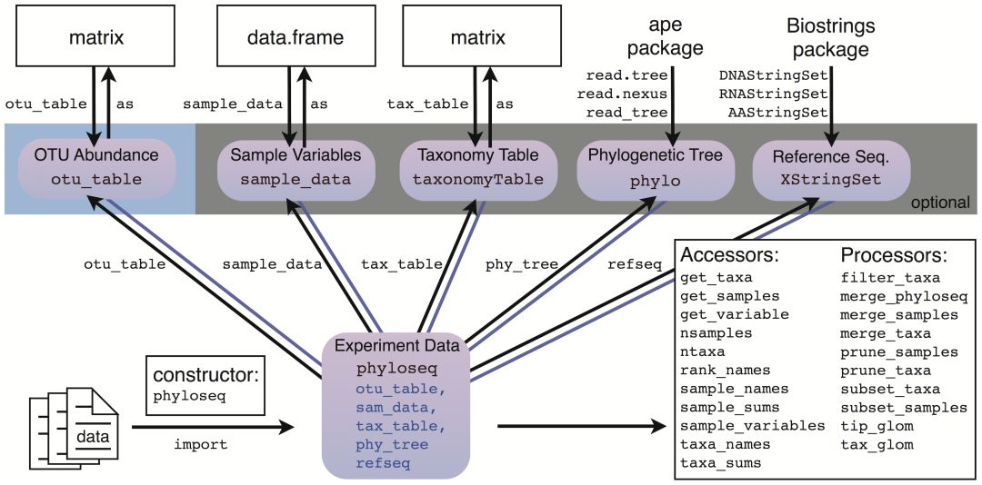
用官网的话说就是:如果你可以将数据导入R中,就可以将其导入phyloseq。主要有五种数据类型,分别是以矩阵形式的otu table和tax(物种注释)文件;数据框形式的mapping文件;另外还有树文件和代表序列文件
数据导入(implot)
构造otu_table
# Create a pretend OTU table that you read from a file, called otumat
otumat = matrix(sample(1:100, 100, replace = TRUE), nrow = 10, ncol = 10)
otumat
rownames(otumat) <- paste0("OTU", 1:nrow(otumat))
colnames(otumat) <- paste0("Sample", 1:ncol(otumat))
otumat
Sample1 Sample2 Sample3 Sample4 Sample5 Sample6 Sample7 Sample8 Sample9 Sample10
OTU1 58 41 93 2 69 4 30 18 81 37
OTU2 45 98 80 96 41 87 74 13 64 41
OTU3 86 11 70 70 82 3 57 43 87 51
OTU4 4 23 22 59 82 82 51 83 40 38
OTU5 64 10 3 58 12 68 25 49 75 78
OTU6 3 85 19 26 19 41 58 21 97 97
OTU7 42 7 17 84 43 22 15 89 4 73
OTU8 13 78 55 65 20 91 5 64 35 43
OTU9 55 89 65 86 44 55 8 82 80 2
OTU10 59 35 8 7 89 62 100 17 34 58构造tax文件
taxmat = matrix(sample(letters, 70, replace = TRUE), nrow = nrow(otumat), ncol = 7)
rownames(taxmat) <- rownames(otumat)
colnames(taxmat) <- c("Domain", "Phylum", "Class", "Order", "Family", "Genus", "Species")
taxmat
Domain Phylum Class Order Family Genus Species
OTU1 "z" "b" "p" "p" "o" "o" "k"
OTU2 "e" "q" "c" "s" "g" "z" "m"
OTU3 "j" "g" "p" "g" "w" "r" "s"
OTU4 "o" "w" "h" "x" "p" "p" "k"
OTU5 "m" "d" "i" "c" "g" "r" "l"
OTU6 "z" "v" "r" "f" "c" "x" "r"
OTU7 "r" "k" "g" "j" "i" "g" "i"
OTU8 "e" "h" "m" "m" "q" "e" "m"
OTU9 "t" "u" "r" "f" "p" "x" "d"
OTU10 "b" "o" "w" "b" "b" "k" "e"otu_table和tax_table函数构造phyloseq对象并加入phyloseq
OTU = otu_table(otumat, taxa_are_rows = TRUE)
TAX = tax_table(taxmat)
OTU
TAX
#加入phyloseq体系
physeq = phyloseq(OTU, TAX)
physeq
格式文件
OTU Table:          [10 taxa and 10 samples]
                     taxa are rows
      Sample1 Sample2 Sample3 Sample4 Sample5 Sample6 Sample7 Sample8 Sample9 Sample10
OTU1       58      41      93       2      69       4      30      18      81       37
· · · · · · ·

Taxonomy Table:     [10 taxa by 7 taxonomic ranks]:
      Domain Phylum Class Order Family Genus Species
OTU1  "z"    "b"    "p"   "p"   "o"    "o"   "k"
· · · · · · ·

phyloseq-class experiment-level object
otu_table()   OTU Table:         [ 10 taxa and 10 samples ]
tax_table()   Taxonomy Table:    [ 10 taxa by 7 taxonomic ranks ]
· · · · · · ·
以科水平做柱状图
默认展示的是count数量
plot_bar(physeq, fill = "Family")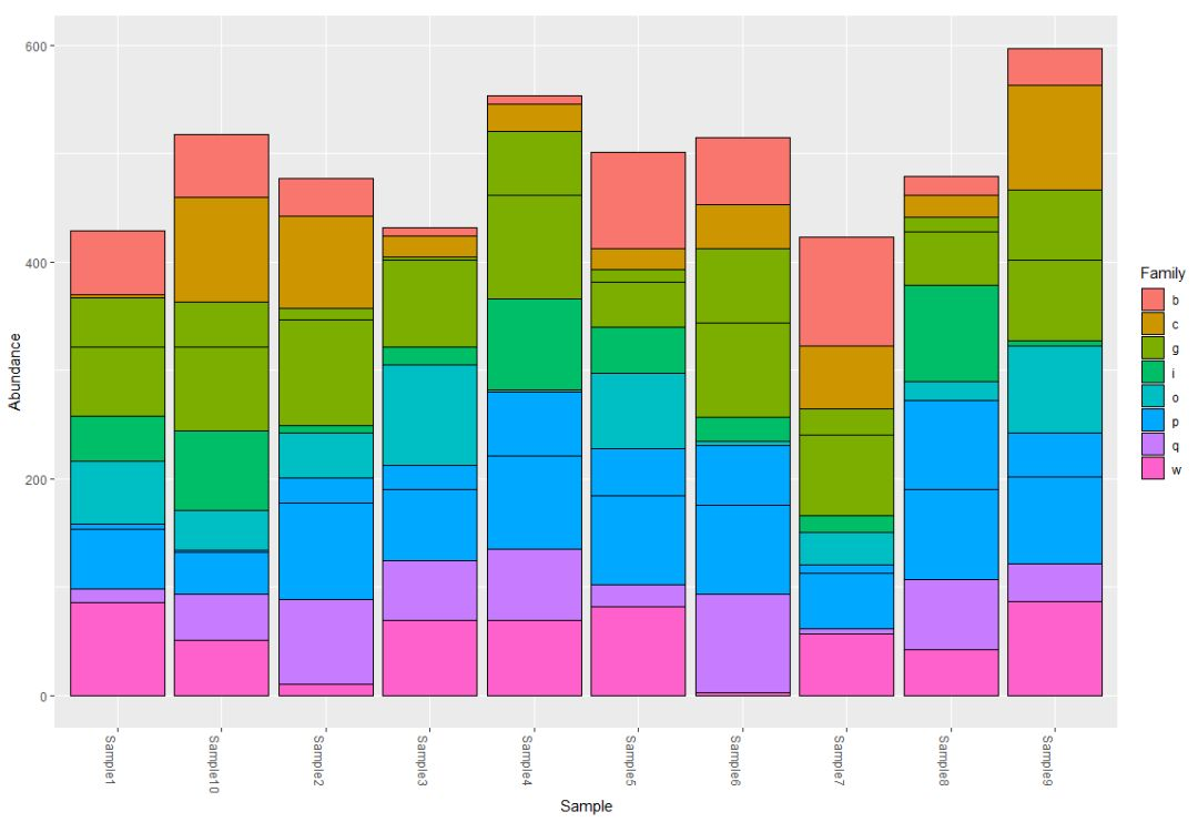
构建样品及其分组文件(mapping)
sampledata = sample_data(data.frame(
  Location = sample(LETTERS[1:4], size=nsamples(physeq), replace=TRUE),
  Depth = sample(50:1000, size=nsamples(physeq), replace=TRUE),
  row.names=sample_names(physeq),
  stringsAsFactors=FALSE
))
sampledata
Sample Data: [10 samples by 2 sample variables]:
Location Depth
Sample1 C 137
Sample2 B 901
Sample3 D 307
Sample4 A 200
Sample5 B 503
Sample6 B 977
Sample7 C 506
Sample8 B 226
Sample9 B 849
Sample10 A 220构建随机树合并phyloseq
library("ape")
random_tree = rtree(ntaxa(physeq), rooted=TRUE, tip.label=taxa_names(physeq))
plot(random_tree)
physeq1 = merge_phyloseq(physeq, sampledata, random_tree)
physeq1
#可重新构建元素
physeq2 = phyloseq(OTU, TAX, sampledata, random_tree)
physeq2
#两者是否相同,很明显是一样的
identical(physeq1, physeq2)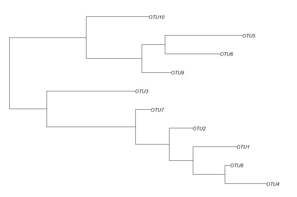
使用phyloseq展示进化树和count丰度热图
plot_tree(physeq1, color="Location", label.tips="taxa_names", ladderize="left", plot.margin=0.3)
plot_tree(physeq1, color="Depth", shape="Location", label.tips="taxa_names", ladderize="right", plot.margin=0.3)
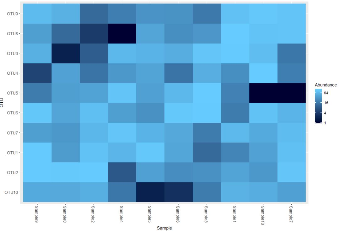
plot_heatmap(physeq1)
plot_heatmap(physeq1, taxa.label="Phylum")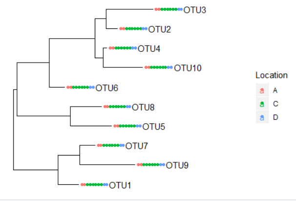
以上部分我们对phyloseq对象及其函数作了一个初步的学习,数据导入部分还有biom格式的较为常见,如有需求,请查看:http://joey711.github.io/phyloseq/import-data.html
boim格式文件导入
#基于biom格式数据导入
rich_dense_biom  = system.file("extdata", "rich_dense_otu_table.biom",  package="phyloseq")
rich_sparse_biom = system.file("extdata", "rich_sparse_otu_table.biom", package="phyloseq")
min_dense_biom   = system.file("extdata", "min_dense_otu_table.biom",   package="phyloseq")
min_sparse_biom  = system.file("extdata", "min_sparse_otu_table.biom",  package="phyloseq")
treefilename = system.file("extdata", "biom-tree.phy",  package="phyloseq")
refseqfilename = system.file("extdata", "biom-refseq.fasta",  package="phyloseq")
import_biom(rich_dense_biom, treefilename, refseqfilename, parseFunction=parse_taxonomy_greengenes)
myData = import_biom(rich_dense_biom, treefilename, refseqfilename, parseFunction=parse_taxonomy_greengenes)
myData
sample_data(myData)
plot_tree(myData, color="Genus", shape="BODY_SITE", size="abundance")
plot_richness(myData, x="BODY_SITE", color="Description")
plot_bar(myData, fill="Genus")
refseq(myData)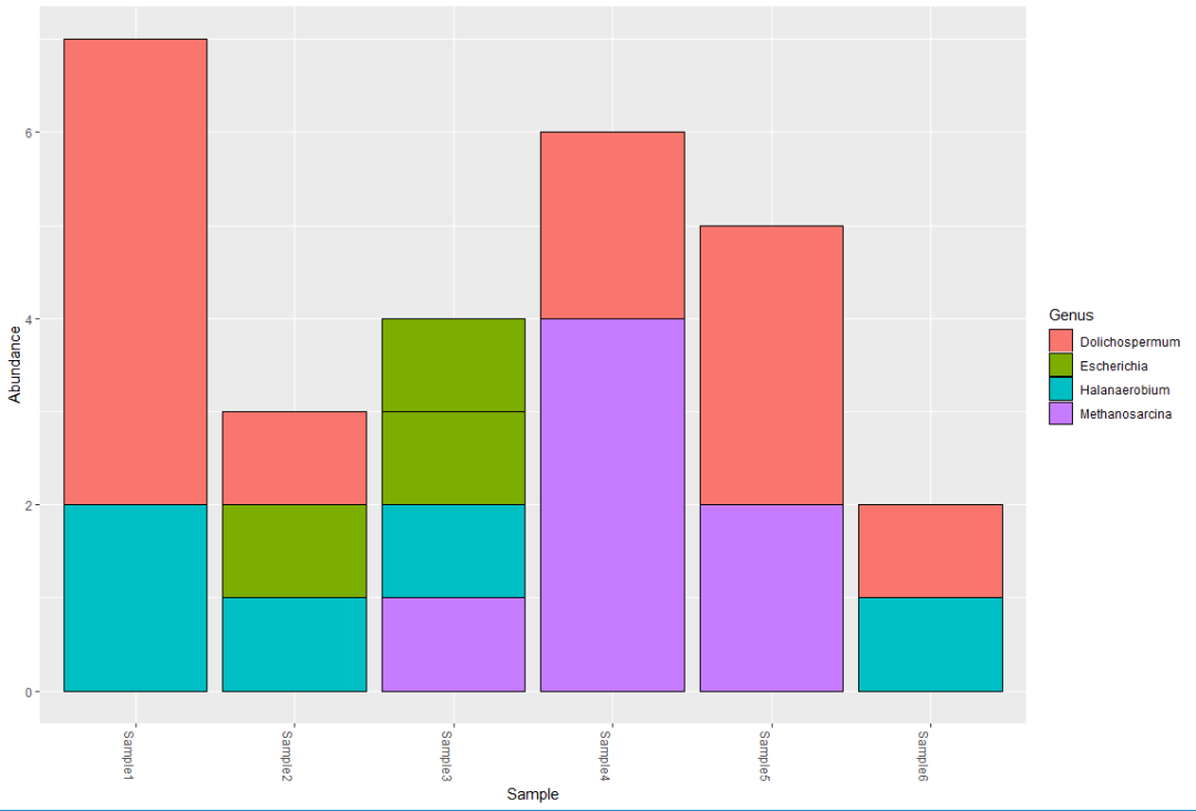
A DNAStringSet instance of length 5
    width seq                                                                                       names
[1]   334 AACGTAGGTCACAAGCGTTGTCCGGAATTACTGGGTGTAAAGG...ACTAGGTGTGGGGGTCTGACCCCTTCCGTGCCGGAGTTAACAC GG_OTU_1
[2]   465 TACGTAGGGAGCAAGCGTTATCCGGATTTATTGGGTGTAAAGG...TTAATTCGAAGCAACGCGAAGAACCTTACCAGGGCTTGACATA GG_OTU_2
[3]   249 TACGTAGGGGGCAAGCGTTATCCGGATTTACTGGGTGTAAAGG...TACTGGACTGTAACTGACGTTGAGGCTCGAAAGCGTGGGGAGC GG_OTU_3
[4]   453 TACGTATGGTGCAAGCGTTATCCGGATTTACTGGGTGTAAAGG...AGCGGTGAGCATGTGGTTAATCGAAGCAACGCGAAGAACCTTA GG_OTU_4
[5]   178 AACGTAGGGTGCAAGCGTTGTCCGGAATTACTGGGTGTAAAGG...GATGGAATTCCCGGTGTAGCGGTGGAATGCGTAGATATCGGGA GG_OTU_5
基于qiime输出文件导入
otufile = system.file("extdata", "GP_otu_table_rand_short.txt.gz", package="phyloseq")
mapfile = system.file("extdata", "master_map.txt", package="phyloseq")
trefile = system.file("extdata", "GP_tree_rand_short.newick.gz", package="phyloseq")
rs_file = system.file("extdata", "qiime500-refseq.fasta", package="phyloseq")
qiimedata = import_qiime(otufile, mapfile, trefile, rs_file)
qiimedata
plot_bar(qiimedata, x="SampleType", fill="Phylum")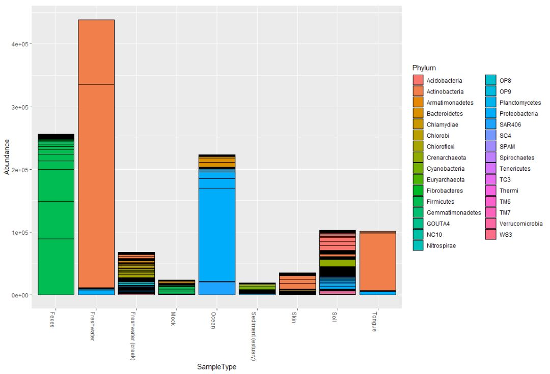
基于其他格式的文件导入参见官网教程:https://joey711.github.io/phyloseq/import-data.html
使用phyloseq的例子
#使用phyloseq
data(GlobalPatterns)
data(esophagus)
data(enterotype)
data(soilrep)
?GlobalPatterns
example(enterotype, ask=FALSE)
?make_network
ig <- make_network(enterotype, "samples", max.dist=0.3)
plot_network(ig, enterotype, color="SeqTech", shape="Enterotype", line_weight=0.3, label=NULL)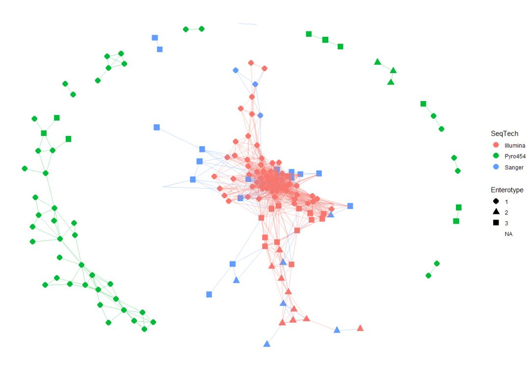
phyloseq按照一定要求合并数据
个人认为phyloseq可以很好的对数据进行清洗,并且连带关系处理的不错 otu丰度信息在合并的OTU表格中是相加的关系
##phyloseq合并数据
data(GlobalPatterns)
GP = GlobalPatterns
#数据过滤,保留count大于0的OTU
GP = prune_taxa(taxa_sums(GlobalPatterns) > 0, GlobalPatterns)
humantypes = c("Feces", "Mock", "Skin", "Tongue")
sample_data(GP)$human <- get_variable(GP, "SampleType") %in% humantypes

#按照SampleType合并样品
mergedGP = merge_samples(GP, "SampleType")
SD = merge_samples(sample_data(GP), "SampleType")
print(SD[, "SampleType"])
sample_data(mergedGP)
OTUnames10 = names(sort(taxa_sums(GP), TRUE)[1:10])
GP10 = prune_taxa(OTUnames10, GP)
mGP10 = prune_taxa(OTUnames10, mergedGP)
ocean_samples = sample_names(subset(sample_data(GP), SampleType=="Ocean"))
print(ocean_samples)
otu_table(GP10)[, ocean_samples]> otu_table(GP10)[, ocean_samples]
OTU Table: [10 taxa and 3 samples]
taxa are rows
NP2 NP3 NP5
329744 91 126 120
317182 3148 12370 63084
549656 5045 10713 1784
279599 113 114 126
360229 16 83 786
94166 49 128 709
550960 11 86 65
158660 13 39 28
331820 24 101 105
189047 4 33 29rowSums(otu_table(GP10)[, ocean_samples])
otu_table(mGP10)["Ocean", ]> otu_table(mGP10)["Ocean", ]
OTU Table: [10 taxa and 1 samples]
taxa are columns
329744 317182 549656 279599 360229 94166 550960 158660 331820 189047
Ocean 337 78602 17542 353 885 886 162 80 230 66plot_richness(GP, "human", "SampleType", title="unmerged")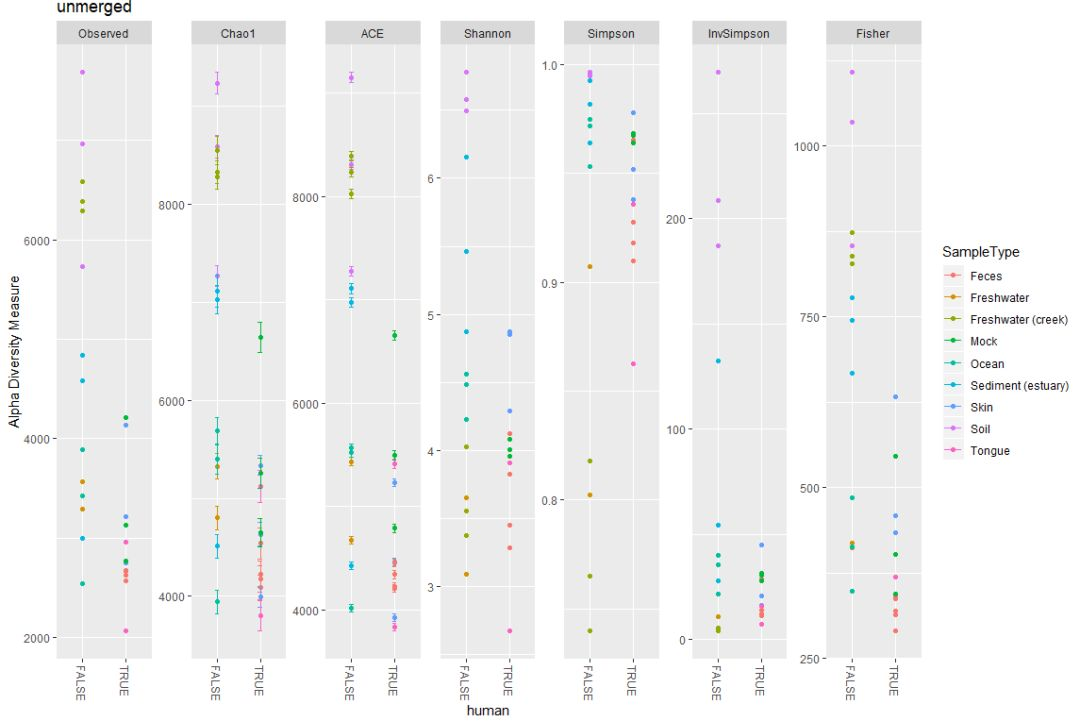
sample_data(mergedGP)$SampleType = sample_names(mergedGP)
sample_data(mergedGP)$human = sample_names(mergedGP) %in% humantypes
plot_richness(mergedGP, "human", "SampleType", title="merged")
根据进化关系对OTU进行合并
load("example-data.RData")
plot_tree(closedps, color="Treatment", size="abundance", sizebase=2, label.tips="taxa_names")

x1 = merge_taxa(closedps, taxa_names(closedps)[3:27], 2)
plot_tree(x1, color="Treatment", size="abundance", sizebase=2, label.tips="taxa_names")
基于phyloseq数据合并
# 数据导出
data(GlobalPatterns)
tree = phy_tree(GlobalPatterns)
tax  = tax_table(GlobalPatterns)
otu  = otu_table(GlobalPatterns)
sam  = sample_data(GlobalPatterns)
# 数据导入
otutax = phyloseq(otu, tax)
otutax

# 合并添加数据
GP2 = merge_phyloseq(otutax, sam, tree)
identical(GP2, GlobalPatterns)
##更加复杂的方式

otusamtree = phyloseq(otu, sam, tree)
GP3 = merge_phyloseq(otusamtree, otutax)
GP3
identical(GP3, GlobalPatterns)

GP4 = merge_phyloseq(otusamtree, tax_table(otutax))
GP4
identical(GP4, GlobalPatterns)
第三部分 访问数据和数据预处理
phyloseq系统内数据查看
##访问数据及其数据处理
data("GlobalPatterns")
GlobalPatterns
#查看OTU数量
ntaxa(GlobalPatterns)
#查看样品数量
nsamples(GlobalPatterns)
#样品名查看,此处查看前五个样品名称
sample_names(GlobalPatterns)[1:5]
#查看tax的分类等级信息
rank_names(GlobalPatterns)
#查看mapping文件表头(样品信息文件列名)
sample_variables(GlobalPatterns)
#查看部分OTU表格矩阵
otu_table(GlobalPatterns)[1:5, 1:5]
#查看部分注释(tax)文件矩阵
tax_table(GlobalPatterns)[1:5, 1:4]
#进化树查看,注意不是可视化
phy_tree(GlobalPatterns)
#查看OTU名称,此处查看前十个
taxa_names(GlobalPatterns)[1:10]

#按照丰度提取前十个OTU,并可视化进化树
myTaxa = names(sort(taxa_sums(GlobalPatterns), decreasing = TRUE)[1:10])
ex1 = prune_taxa(myTaxa, GlobalPatterns)
plot(phy_tree(ex1), show.node.label = TRUE)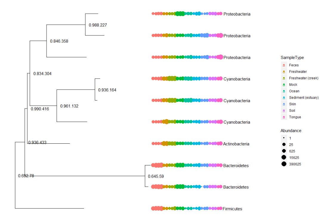
数据的预处理
#数据预处理
#转化OTUcount数为相对丰度
GPr = transform_sample_counts(GlobalPatterns, function(x) x / sum(x) )
otu_table(GPr)[1:5][1:5]
#提取丰度大于十万份之一的OTU
GPfr = filter_taxa(GPr, function(x) mean(x) > 1e-5, TRUE)
#提取指定分类的OTU
GP.chl = subset_taxa(GlobalPatterns, Phylum=="Chlamydiae")
#提取总count数量大于20的样品
GP.chl = prune_samples(sample_sums(GP.chl)>=20, GP.chl)
#合并指定OTU:taxa_names(GP.chl)[1:5]为一个OTU
GP.chl.merged = merge_taxa(GP.chl, taxa_names(GP.chl)[1:5])
# gpsfbg = tax_glom(gpsfb, "Family")
# plot_tree(gpsfbg, color="SampleType", shape="Class", size="abundance")
transform_sample_counts(GP.chl, function(OTU) OTU/sum(OTU) )
#去除至少20%样本中未见过3次以上的OTU,注意编写函数的形式
GP = filter_taxa(GlobalPatterns, function(x) sum(x > 3) > (0.2*length(x)), TRUE)
#对样品分组文件mapping添加一列
sample_data(GP)$human = factor( get_variable(GP, "SampleType") %in% c("Feces", "Mock", "Skin", "Tongue") )
#测序深度进行统一
total = median(sample_sums(GP))
standf = function(x, t=total) round(t * (x / sum(x)))
gps = transform_sample_counts(GP, standf)
sample_sums(gps)
#变异系数过滤OTU,减少一些意外OTU误差
gpsf = filter_taxa(gps, function(x) sd(x)/mean(x) > 3.0, TRUE)
#提取指定门类OTU
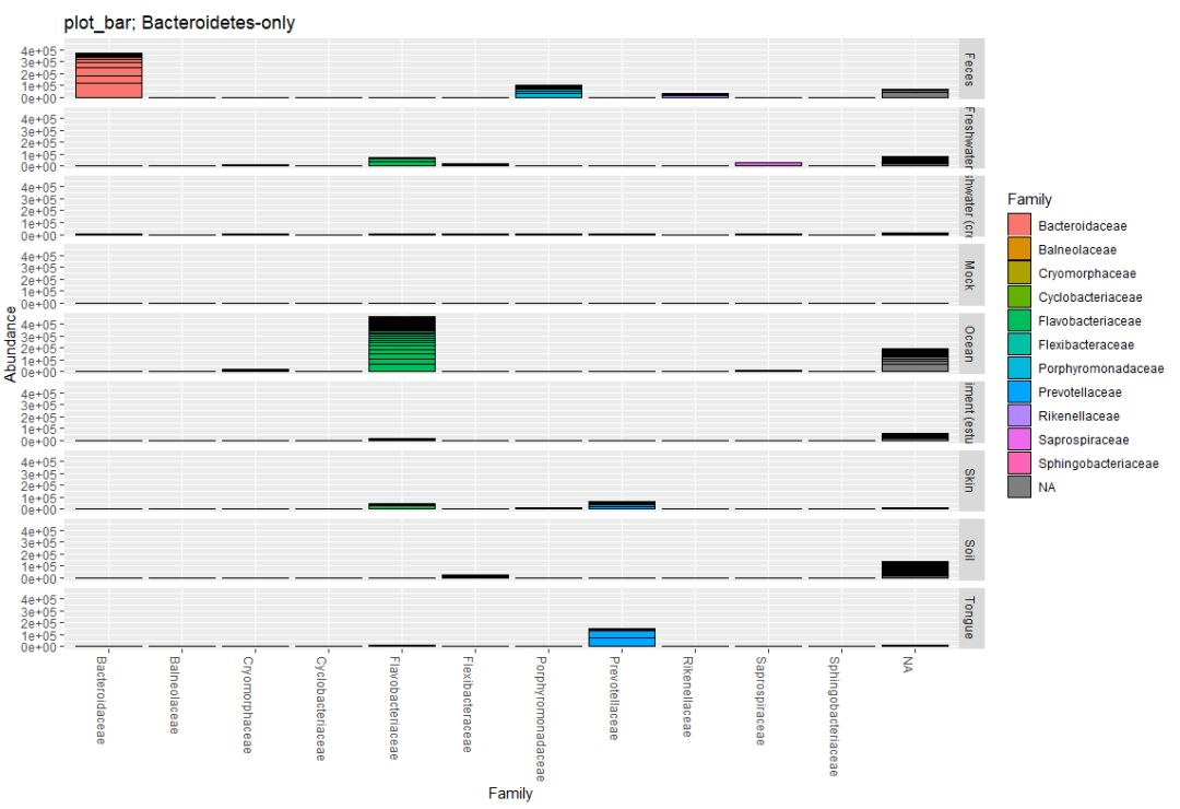
gpsfb = subset_taxa(gpsf, Phylum=="Bacteroidetes")
title = "plot_bar; Bacteroidetes-only"
plot_bar(gpsfb, "SampleType", "Abundance", title=title)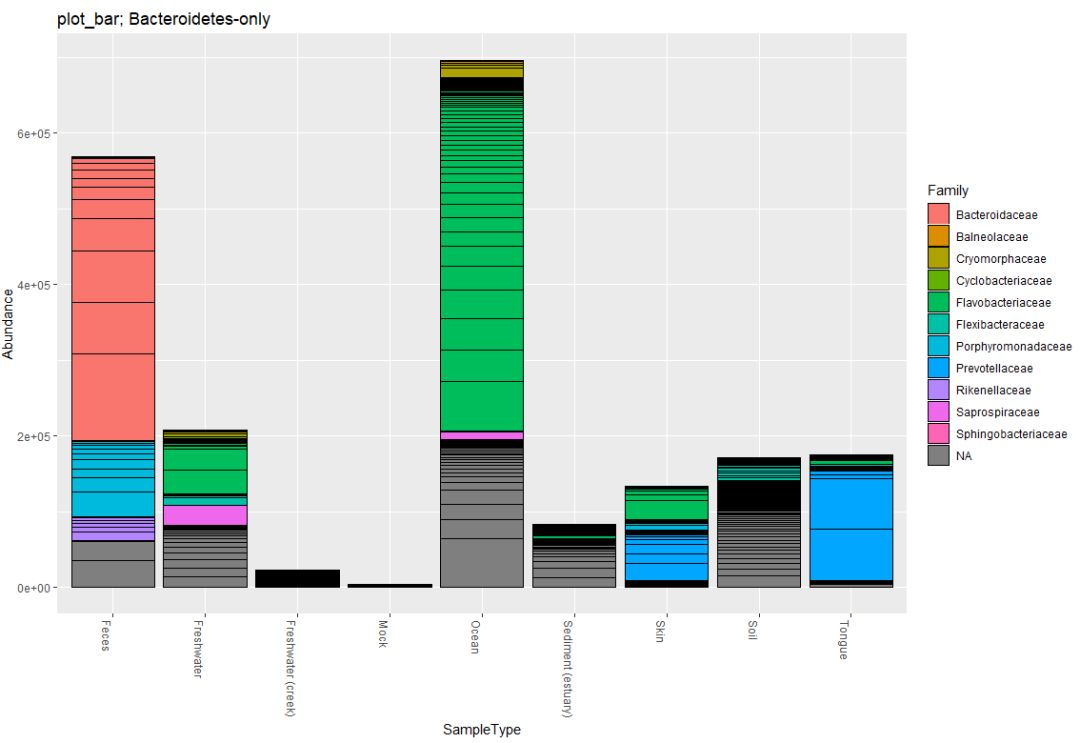
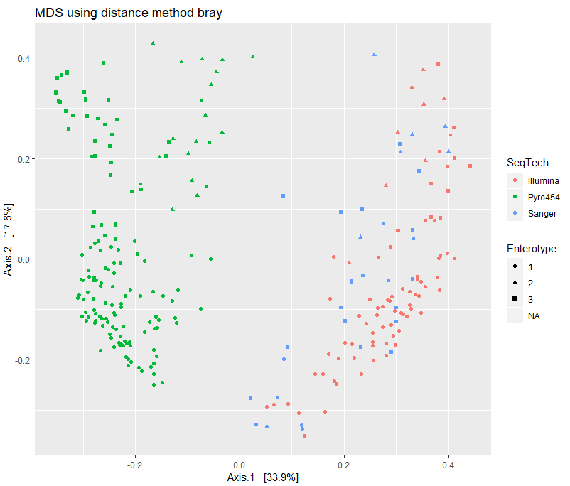
基于微生物群落数据距离的计算
##基于phyloseq的微生物群落聚类的计算
library("plyr"); packageVersion("plyr")
data(enterotype)
enterotype <- subset_taxa(enterotype, Genus != "-1")
#我们进行查看发现有很多的距离算法
dist_methods <- unlist(distanceMethodList)
print(dist_methods)
#删除需要tree的距离算法
# Remove them from the vector
dist_methods <- dist_methods[-(1:3)]
# 删除需要用户自定义的距离算法
dist_methods["designdist"]
dist_methods = dist_methods[-which(dist_methods=="ANY")]

plist <- vector("list", length(dist_methods))
names(plist) = dist_methods
for( i in dist_methods ){
  # Calculate distance matrix
  iDist <- distance(enterotype, method=i)
  # Calculate ordination
  iMDS  <- ordinate(enterotype, "MDS", distance=iDist)
  ## Make plot
  # Don't carry over previous plot (if error, p will be blank)
  p <- NULL
  # Create plot, store as temp variable, p
  p <- plot_ordination(enterotype, iMDS, color="SeqTech", shape="Enterotype")
  # Add title to each plot
  p <- p + ggtitle(paste("MDS using distance method ", i, sep=""))
  # Save the graphic to file.
  plist[[i]] = p
}

df = ldply(plist, function(x) x$data)
names(df)[1] <- "distance"
p = ggplot(df, aes(Axis.1, Axis.2, color=SeqTech, shape=Enterotype))
p = p + geom_point(size=3, alpha=0.5)
p = p + facet_wrap(~distance, scales="free")
p = p + ggtitle("MDS on various distance metrics for Enterotype dataset")
p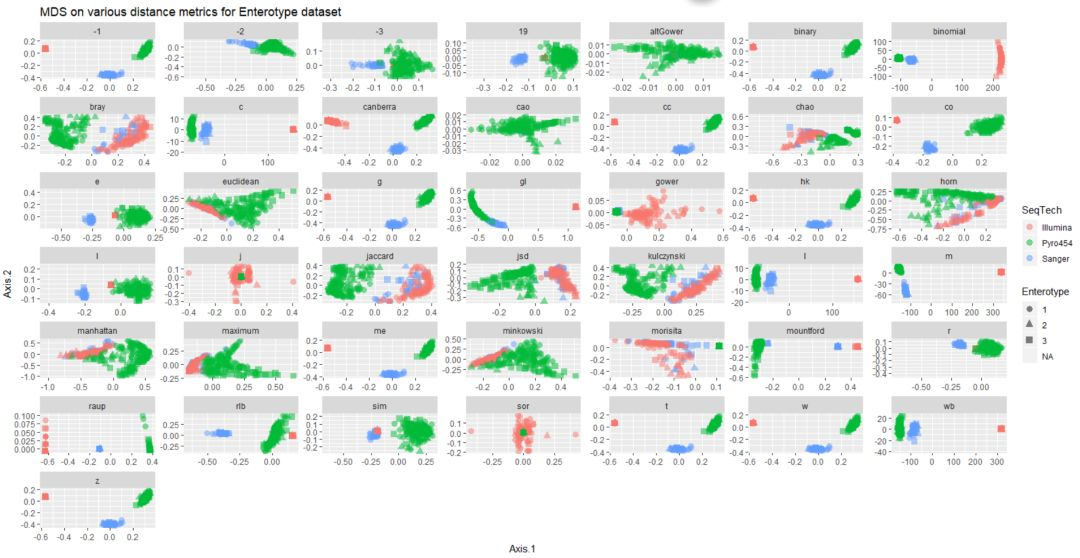
df = ldply(plist, function(x) x$data)
names(df)[1] <- "distance"
p = ggplot(df, aes(Axis.1, Axis.2, color=Enterotype, shape=SeqTech))
p = p + geom_point(size=3, alpha=0.5)
p = p + facet_wrap(~distance, scales="free")
p = p + ggtitle("MDS on various distance metrics for Enterotype dataset")
p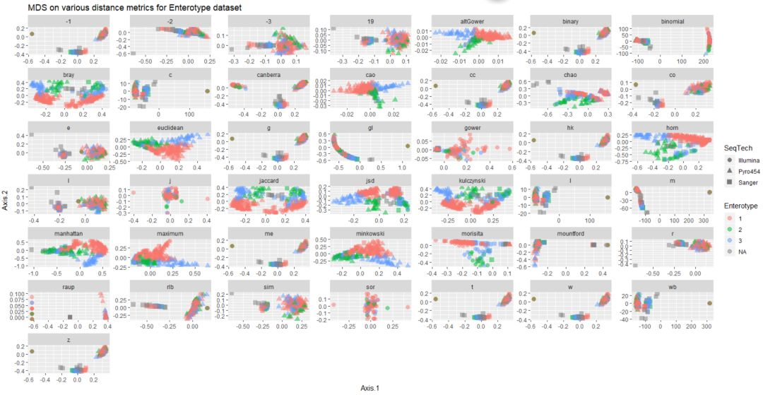
#jsd距离查看效果
print(plist[["jsd"]])
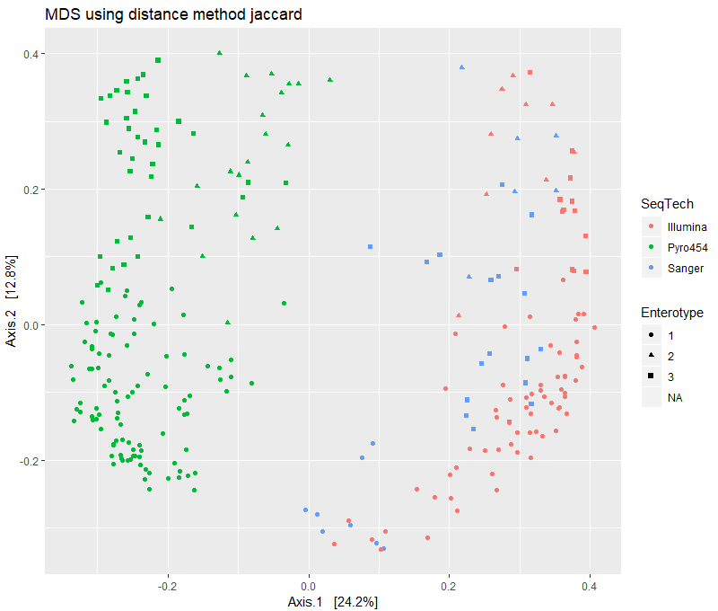
print(plist[["jaccard"]])
print(plist[["bray"]])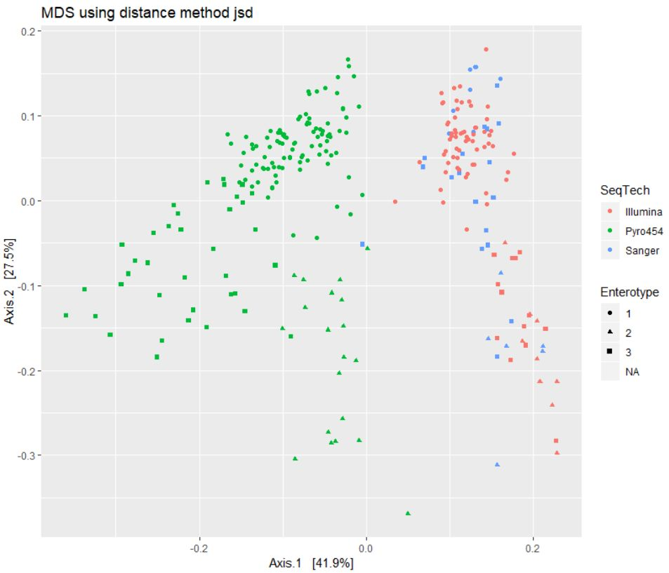
差异统计
library("phyloseq"); packageVersion("phyloseq")
library("cluster"); packageVersion("cluster")
library("ggplot2"); packageVersion("ggplot2")
##统计差异
theme_set(theme_bw())
# Load data
data(enterotype)
#jsd距离进行MDS排序
exord = ordinate(enterotype, method="MDS", distance="jsd")

pam1 = function(x, k){list(cluster = pam(x,k, cluster.only=TRUE))}
x = phyloseq:::scores.pcoa(exord, display="sites")
# gskmn = clusGap(x[, 1:2], FUN=kmeans, nstart=20, K.max = 6, B = 500)
gskmn = clusGap(x[, 1:2], FUN=pam1, K.max = 6, B = 50)

gap_statistic_ordination = function(ord, FUNcluster, type="sites", K.max=6, axes=c(1:2), B=500, verbose=interactive(), ...){
  require("cluster")
  #   If "pam1" was chosen, use this internally defined call to pam
  if(FUNcluster == "pam1"){
    FUNcluster = function(x,k) list(cluster = pam(x, k, cluster.only=TRUE))
  }
  # Use the scores function to get the ordination coordinates
  x = phyloseq:::scores.pcoa(ord, display=type)
  #   If axes not explicitly defined (NULL), then use all of them
  if(is.null(axes)){axes = 1:ncol(x)}
  #   Finally, perform, and return, the gap statistic calculation using cluster::clusGap
  clusGap(x[, axes], FUN=FUNcluster, K.max=K.max, B=B, verbose=verbose, ...)
}

plot_clusgap = function(clusgap, title="Gap Statistic calculation results"){
  require("ggplot2")
  gstab = data.frame(clusgap$Tab, k=1:nrow(clusgap$Tab))
  p = ggplot(gstab, aes(k, gap)) + geom_line() + geom_point(size=5)
  p = p + geom_errorbar(aes(ymax=gap+SE.sim, ymin=gap-SE.sim))
  p = p + ggtitle(title)
  return(p)
}

gs = gap_statistic_ordination(exord, "pam1", B=50, verbose=FALSE)
print(gs, method="Tibs2001SEmax")

plot_clusgap(gs)

plot(gs, main = "Gap statistic for the 'Enterotypes' data")
mtext("Looks like 4 clusters is best, with 3 and 5 close runners up.")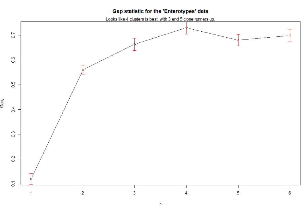
猜你喜欢
10000+:菌群分析 宝宝与猫狗 梅毒狂想曲 提DNA发Nature Cell专刊 肠道指挥大脑
文献阅读 热心肠 SemanticScholar Geenmedical
16S功能预测 PICRUSt FAPROTAX Bugbase Tax4Fun
生物科普: 肠道细菌 人体上的生命 生命大跃进 细胞暗战 人体奥秘
写在后面
为鼓励读者交流、快速解决科研困难,我们建立了“宏基因组”专业讨论群,目前己有国内外5000+ 一线科研人员加入。参与讨论,获得专业解答,欢迎分享此文至朋友圈,并扫码加主编好友带你入群,务必备注“姓名-单位-研究方向-职称/年级”。PI请明示身份,另有海内外微生物相关PI群供大佬合作交流。技术问题寻求帮助,首先阅读《如何优雅的提问》学习解决问题思路,仍未解决群内讨论,问题不私聊,帮助同行。

学习16S扩增子、宏基因组科研思路和分析实战,关注“宏基因组”
 点击阅读原文,跳转最新文章目录阅读


 1万+
1万+

 被折叠的 条评论
为什么被折叠?
被折叠的 条评论
为什么被折叠?
 到【灌水乐园】发言


