【点云处理】点云法向量估计及其加速(3)

        接上篇【点云处理】点云法向量估计及其加速(2)。在上一篇文章中，我们直接使用pcl的NormalEstimation和NormalEstimationOMP来计算点云表面法向量都存在明显的效率问题。其中NormalEstimation没有用到多核多线程性能自然低，但NormalEstimationOMP使用到了多核多线程也并没有取得加速效果。纵观点云法线的计算过程，耗时主要几种在两处运算。一个是计算每一个点云的K近邻，另一处就是紧接着的计算法向量。这两处运算其实都明显具有可GPU并行计算的特点，考虑到PCL已经直接支持GPU计算法向量，我们先尝试使用PCL提供的GPU计算法向量的API。

使用PCL GPU计算点云法线

【示例代码】

#include <time.h>
#include <cmath>
#include <functional>
#include <ros/ros.h>
#include <sensor_msgs/PointCloud2.h>
#include <pcl/console/time.h>
#include <pcl/kdtree/kdtree.h>
#include<pcl/gpu/features/features.hpp>
#include <pcl/features/normal_3d_omp.h>
#include <pcl_conversions/pcl_conversions.h>

int main(int argc, char** argv) {
    ros::init(argc, argv, "n_lidar_gpu_normal");
    ros::NodeHandle node;
    pcl::PointCloud<pcl::PointXYZ>::Ptr cloud(new pcl::PointCloud<pcl::PointXYZ>);

    const boost::function<void (const boost::shared_ptr<sensor_msgs::PointCloud2 const>&)> callback =[&](sensor_msgs::PointCloud2::ConstPtr msg_pc_ptr) {
        pcl::fromROSMsg(*msg_pc_ptr, *cloud);
        
        auto t1 = clock();
        pcl::KdTreeFLANN<pcl::PointXYZ>::Ptr kdtree(new pcl::KdTreeFLANN<pcl::PointXYZ>);
        kdtree->setInputCloud(cloud);

        size_t cloud_size = cloud->size();
        std::vector<std::vector<int>> neighbors_all(cloud_size);
        std::vector<int> sizes(cloud_size);
        std::vector<float> dists;
        for (auto i=0; i<cloud_size; i++) {
            kdtree->nearestKSearch(cloud->points[i], 10, neighbors_all[i], dists);
            sizes[i] = neighbors_all[i].size();
        }
        auto t2 = clock();
        auto knn_time = (float)((t2-t1)*1000/CLOCKS_PER_SEC);

        int max_nn_size = *max_element(sizes.begin(), sizes.end());
        std::vector<int> temp_neighbors_all(max_nn_size * cloud_size);
        pcl::gpu::PtrStep<int> ps(&temp_neighbors_all[0], max_nn_size * pcl::gpu::PtrStep<int>::elem_size);
	    for (size_t i=0; i<cloud->size(); ++i) {
		    std::copy(neighbors_all[i].begin(), neighbors_all[i].end(), ps.ptr(i));
        }

        pcl::gpu::NeighborIndices gpu_neighbor_indices;
        pcl::gpu::NormalEstimation::PointCloud gpu_cloud;
        gpu_cloud.upload(cloud->points);
        gpu_neighbor_indices.upload(temp_neighbors_all, sizes, max_nn_size);

        pcl::gpu::NormalEstimation::Normals gpu_normals;
	    pcl::gpu::NormalEstimation::computeNormals(gpu_cloud, gpu_neighbor_indices, gpu_normals);
	    pcl::gpu::NormalEstimation::flipNormalTowardsViewpoint(gpu_cloud, 0.f, 0.f, 0.f, gpu_normals);
        auto t3 = clock();
        auto compute_normal_time = (float)((t3-t2)*1000/CLOCKS_PER_SEC);

	    std::vector<pcl::PointXYZ> normals;
	    gpu_normals.download(normals);

        auto t4 = clock();
        auto total_time = (float)((t4-t1)*1000/CLOCKS_PER_SEC);
        printf("cloud size:%zu, knn_time:%.2f ms,compute_normal_time:%.2f ms, total_time:%.2f ms\n", cloud->size(), knn_time, compute_normal_time, total_time);
    };
    ros::Subscriber pc_sub = node.subscribe<sensor_msgs::PointCloud2>("/BackLidar/lslidar_point_cloud", 1, callback);
    ros::spin();
    return 0;
}

【运行结果】

cloud size:26791, knn_time:141.00 ms,compute_normal_time:3.00 ms, total_time:145.00 ms
cloud size:32185, knn_time:192.00 ms,compute_normal_time:5.00 ms, total_time:198.00 ms
cloud size:25446, knn_time:132.00 ms,compute_normal_time:3.00 ms, total_time:135.00 ms
cloud size:26707, knn_time:144.00 ms,compute_normal_time:3.00 ms, total_time:148.00 ms
cloud size:25125, knn_time:131.00 ms,compute_normal_time:3.00 ms, total_time:134.00 ms
cloud size:50287, knn_time:269.00 ms,compute_normal_time:6.00 ms, total_time:276.00 ms
cloud size:87313, knn_time:464.00 ms,compute_normal_time:11.00 ms, total_time:477.00 ms
cloud size:37661, knn_time:205.00 ms,compute_normal_time:5.00 ms, total_time:210.00 ms
cloud size:32271, knn_time:164.00 ms,compute_normal_time:3.00 ms, total_time:169.00 ms
cloud size:6450, knn_time:31.00 ms,compute_normal_time:1.00 ms, total_time:33.00 ms

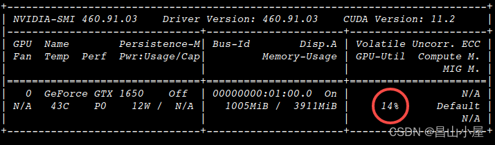
total_time为单帧点云的计算时间，可见相比NomalEstimation和NormalEstimationOMP在我的实验平台上有将近10倍的加速效果。而此时GPU的利用率也仅仅不到20%。

 这个也好理解，对总的时间分段分析可知。当前的瓶颈已经落在了K近邻的计算上。so，如何优化k近邻的计算是下一步工作的重点。