


简 介
CART模型,即Classification And Regression Trees。它和一般回归分析类似,是用来对变量进行解释和预测的工具,也是数据挖掘中的一种常用算法。如果因变量是连续数据,相对应的分析称为回归树,如果因变量是分类数据,则相应的分析称为分类树。
决策树是一种倒立的树结构,它由内部节点、叶子节点和边组成。其中最上面的一个节点叫根节点。 构造一棵决策树需要一个训练集,一些例子组成,每个例子用一些属性(或特征)和一个类别标记来描述。构造决策树的目的是找出属性和类别间的关系,一旦这种关系找出,就能用它来预测将来未知类别的记录的类别。这种具有预测功能的系统叫决策树分类器。其算法的优点在于:
1)可以生成可以理解的规则。
2)计算量相对来说不是很大。
3)可以处理多种数据类型。
4)决策树可以清晰的显示哪些变量较重要。

软件包安装
这里我们主要介绍caret,另外还有两个包同样可以实现 Bagged CART 算法,软件包安装方法如下:
if(require(caret))
  install.packages("caret")
数据读取
这里我们选择之前在分析机器学习是曾经使用过的数据集:BreastCancer,可以跟我们之前的方法对比一下:
library(caret)
BreastCancer <- read.csv("wisc_bc_data.csv", stringsAsFactors = FALSE)
BreastCancer = BreastCancer[, -1]
dim(BreastCancer)
## [1] 568  31
str(BreastCancer)
## 'data.frame':	568 obs. of  31 variables:
##  $ diagnosis              : chr  "M" "M" "M" "M" ...
##  $ radius_mean            : num  20.6 19.7 11.4 20.3 12.4 ...
##  $ texture_mean           : num  17.8 21.2 20.4 14.3 15.7 ...
##  $ perimeter_mean         : num  132.9 130 77.6 135.1 82.6 ...
##  $ area_mean              : num  1326 1203 386 1297 477 ...
##  $ smoothness_mean        : num  0.0847 0.1096 0.1425 0.1003 0.1278 ...
##  $ compactne_mean         : num  0.0786 0.1599 0.2839 0.1328 0.17 ...
##  $ concavity_mean         : num  0.0869 0.1974 0.2414 0.198 0.1578 ...
##  $ concave_points_mean    : num  0.0702 0.1279 0.1052 0.1043 0.0809 ...
##  $ symmetry_mean          : num  0.181 0.207 0.26 0.181 0.209 ...
##  $ fractal_dimension_mean : num  0.0567 0.06 0.0974 0.0588 0.0761 ...
##  $ radius_se              : num  0.543 0.746 0.496 0.757 0.335 ...
##  $ texture_se             : num  0.734 0.787 1.156 0.781 0.89 ...
##  $ perimeter_se           : num  3.4 4.58 3.44 5.44 2.22 ...
##  $ area_se                : num  74.1 94 27.2 94.4 27.2 ...
##  $ smoothness_se          : num  0.00522 0.00615 0.00911 0.01149 0.00751 ...
##  $ compactne_se           : num  0.0131 0.0401 0.0746 0.0246 0.0335 ...
##  $ concavity_se           : num  0.0186 0.0383 0.0566 0.0569 0.0367 ...
##  $ concave_points_se      : num  0.0134 0.0206 0.0187 0.0188 0.0114 ...
##  $ symmetry_se            : num  0.0139 0.0225 0.0596 0.0176 0.0216 ...
##  $ fractal_dimension_se   : num  0.00353 0.00457 0.00921 0.00511 0.00508 ...
##  $ radius_worst           : num  25 23.6 14.9 22.5 15.5 ...
##  $ texture_worst          : num  23.4 25.5 26.5 16.7 23.8 ...
##  $ perimeter_worst        : num  158.8 152.5 98.9 152.2 103.4 ...
##  $ area_worst             : num  1956 1709 568 1575 742 ...
##  $ smoothness_worst       : num  0.124 0.144 0.21 0.137 0.179 ...
##  $ compactne_worst        : num  0.187 0.424 0.866 0.205 0.525 ...
##  $ concavity_worst        : num  0.242 0.45 0.687 0.4 0.535 ...
##  $ concave_points_worst   : num  0.186 0.243 0.258 0.163 0.174 ...
##  $ symmetry_worst         : num  0.275 0.361 0.664 0.236 0.399 ...
##  $ fractal_dimension_worst: num  0.089 0.0876 0.173 0.0768 0.1244 ...
table(BreastCancer$diagnosis)
##
##   B   M
## 357 211
基于机器学习构建临床预测模型
MachineLearning 2. 因子分析(Factor Analysis)
MachineLearning 3. 聚类分析(Cluster Analysis)
MachineLearning 4. 癌症诊断方法之 K-邻近算法(KNN)
MachineLearning 5. 癌症诊断和分子分型方法之支持向量机(SVM)
MachineLearning 6. 癌症诊断机器学习之分类树(Classification Trees)
MachineLearning 7. 癌症诊断机器学习之回归树(Regression Trees)
MachineLearning 8. 癌症诊断机器学习之随机森林(Random Forest)
MachineLearning 9. 癌症诊断机器学习之梯度提升算法(Gradient Boosting)
MachineLearning 10. 癌症诊断机器学习之神经网络(Neural network)
MachineLearning 11. 机器学习之随机森林生存分析(randomForestSRC)
MachineLearning 12. 机器学习之降维方法t-SNE及可视化 (Rtsne)
MachineLearning 13. 机器学习之降维方法UMAP及可视化 (umap)
MachineLearning 14. 机器学习之集成分类器(AdaBoost)
MachineLearning 15. 机器学习之集成分类器(LogitBoost)
MachineLearning 16. 机器学习之梯度提升机(GBM)
MachineLearning 17. 机器学习之围绕中心点划分算法(PAM)
MachineLearning 18. 机器学习之贝叶斯分类器(Naive Bayes)
MachineLearning 19. 机器学习之神经网络分类器(NNET)
实例操作
数据预处理
数据预处理包括五个部,先判断数据是否有缺失,缺失数量,在进行如下步骤:
删除低方差的变量
删欧与其它自变最有很强相关性的变最
去除多重共线性
对数据标准化处理,并补足缺失值
特征筛选,递归特征消除法(RFE)
# 删除方差为0的变量
zerovar = nearZeroVar(BreastCancer[, -1])
zerovar
## integer(0)
# BreastCancer=BreastCancer[,-zerovar]

# 首先删除强相关的变量
descrCorr = cor(BreastCancer[, -1])
descrCorr[1:5, 1:5]
##                 radius_mean texture_mean perimeter_mean area_mean
## radius_mean       1.0000000   0.32938305      0.9978764 0.9873442
## texture_mean      0.3293830   1.00000000      0.3359176 0.3261929
## perimeter_mean    0.9978764   0.33591759      1.0000000 0.9865482
## area_mean         0.9873442   0.32619289      0.9865482 1.0000000
## smoothness_mean   0.1680940  -0.01776898      0.2045046 0.1748380
##                 smoothness_mean
## radius_mean          0.16809398
## texture_mean        -0.01776898
## perimeter_mean       0.20450464
## area_mean            0.17483805
## smoothness_mean      1.00000000
highCorr = findCorrelation(descrCorr, 0.9)
highCorr
##  [1]  7  8 23 21  3 24  1 13 14  2
BreastCancer = BreastCancer[, -(highCorr + 1)]
dim(BreastCancer)
## [1] 568  21
# 随后解决多重共线性,本例中不存在多重共线性问题
comboInfo = findLinearCombos(BreastCancer[, -1])
comboInfo
## $linearCombos
## list()
##
## $remove
## NULL
# BreastCancer=BreastCancer[, -(comboInfo$remove+2)]
Process = preProcess(BreastCancer)
Process
## Created from 568 samples and 21 variables
##
## Pre-processing:
##   - centered (20)
##   - ignored (1)
##   - scaled (20)
BreastCancer = predict(Process, BreastCancer)
特征选择
在进行数据挖掘时,我们并不需要将所有的自变量用来建模,而是从中选择若干最重要的变量,这称为特征选择(feature selection)。一种算法就是后向选择,即先将所有的变量都包括在模型中,然后计算其效能(如误差、预测精度)和变量重要排序,然后保留最重要的若干变量,再次计算效能,这样反复迭代,找出合适的自变量数目。这种算法的一个缺点在于可能会存在过度拟合,所以需要在此算法外再套上一个样本划分的循环。在caret包中的rfe命令可以完成这项任务。 functions是确定用什么样的模型进行自变量排序,包括:
随机森林rfFuncs,
lmFuncs(线性回归),
nbFuncs(朴素贝叶斯),
treebagFuncs(装袋决策树),
caretFuncs(自定义的训练模型)。
method是确定抽样方法,cv即交叉检验, 还有提升boot以及留一交叉检验LOOCV。
ctrl = rfeControl(functions = caretFuncs, method = "repeatedcv", verbose = FALSE,
    returnResamp = "final")
BreastCancer$diagnosis = as.factor(BreastCancer$diagnosis)
Profile = rfe(BreastCancer[, -1], BreastCancer$diagnosis, rfeControl = ctrl)
print(Profile)
##
## Recursive feature selection
##
## Outer resampling method: Cross-Validated (10 fold, repeated 1 times)
##
## Resampling performance over subset size:
##
##  Variables Accuracy  Kappa AccuracySD KappaSD Selected
##          4   0.9332 0.8566    0.03596 0.07796
##          8   0.9561 0.9050    0.02513 0.05479
##         16   0.9578 0.9083    0.03429 0.07471
##         20   0.9596 0.9117    0.04219 0.09263        *
##
## The top 5 variables (out of 20):
##    concave_points_worst, area_mean, concavity_worst, radius_se, compactne_worst
plot(Profile)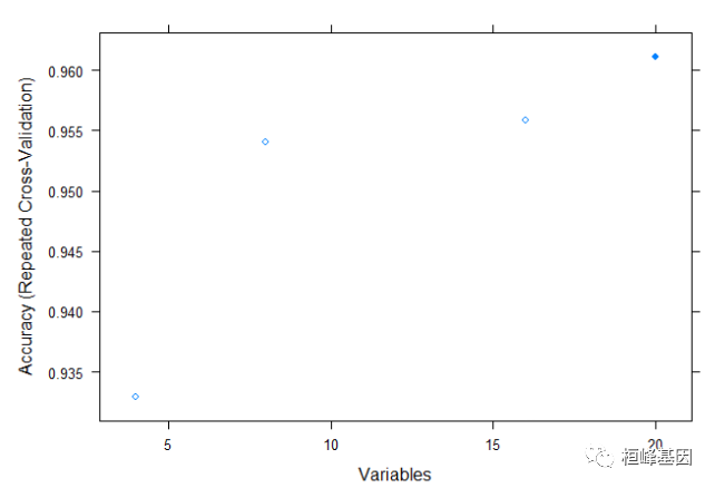
xyplot(Profile$results$Kappa ~ Profile$results$Variables, ylab = "Kappa", xlab = "Variables",
    type = c("g", "p", "l"), auto.key = TRUE)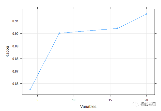
xyplot(Profile$results$Accuracy ~ Profile$results$Variables, ylab = "Accuracy", xlab = "Variables",
    type = c("g", "p", "l"), auto.key = TRUE)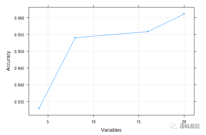
数据分割
数据分割就是将数据分割为测试数据集和验证数据集,关于这个数据分割可以参考Topic 5. 样本量确定及分割,具体操作如下:
library(tidyverse)
library(sampling)
set.seed(123)
# 每层抽取70%的数据
train_id <- strata(BreastCancer, "diagnosis", size = rev(round(table(BreastCancer$diagnosis) *
0.7)))$ID_unit
# 训练数据
trainData <- BreastCancer[train_id, ]
# 测试数据
testData <- BreastCancer[-train_id, ]
# 查看训练、测试数据中正负样本比例
prop.table(table(trainData$diagnosis))
##
## B M
## 0.6281407 0.3718593
prop.table(table(testData$diagnosis))
##
## B M
## 0.6294118 0.3705882
prop.table(table(BreastCancer$diagnosis))
##
## B M
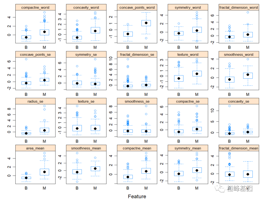
## 0.6285211 0.3714789可视化重要变量
我们可以使用featurePlot()函数可视化每个自变量的取值范围以及不同分类比较等问题。
对于分类模型选择:box, strip, density, pairs or ellipse
对于回归模型选择:pairs or scatter
#4. How to visualize the importance of variables using featurePlot()
featurePlot(x = trainData[, 2:21],
            y = as.factor(trainData$diagnosis),
            plot = "box", #For classification:box, strip, density, pairs or ellipse. For regression, pairs or scatter
            strip=strip.custom(par.strip.text=list(cex=.7)),
            scales = list(x = list(relation="free"),
                          y = list(relation="free"))
)
定义测试参数
在正式训练前,首先需要使用trainControl函数定义模型训练参数,method确定多次交叉检验的抽样方法,number确定了划分的重数, repeats确定了反复次数。
fitControl <- trainControl(
  method = 'cv',                   # k-fold cross validation
  number = 5,                      # number of folds
  savePredictions = 'final',       # saves predictions for optimal tuning parameter
  classProbs = T,                  # should class probabilities be returned
  summaryFunction=twoClassSummary  # results summary function
)
构建袋装决策树分类器
使用train训练模型,本例中使用的时神经网络算法,我们可以对一些参数进行手动调优,包括interaction.depth,n.trees,shrinkage,n.minobsinnode等参数,也可以使用默认参数
names(getModelInfo())
##   [1] "ada"                 "AdaBag"              "AdaBoost.M1"
##   [4] "adaboost"            "amdai"               "ANFIS"
##   [7] "avNNet"              "awnb"                "awtan"
##  [10] "bag"                 "bagEarth"            "bagEarthGCV"
##  [13] "bagFDA"              "bagFDAGCV"           "bam"
##  [16] "bartMachine"         "bayesglm"            "binda"
##  [19] "blackboost"          "blasso"              "blassoAveraged"
##  [22] "bridge"              "brnn"                "BstLm"
##  [25] "bstSm"               "bstTree"             "C5.0"
##  [28] "C5.0Cost"            "C5.0Rules"           "C5.0Tree"
##  [31] "cforest"             "chaid"               "CSimca"
##  [34] "ctree"               "ctree2"              "cubist"
##  [37] "dda"                 "deepboost"           "DENFIS"
##  [40] "dnn"                 "dwdLinear"           "dwdPoly"
##  [43] "dwdRadial"           "earth"               "elm"
##  [46] "enet"                "evtree"              "extraTrees"
##  [49] "fda"                 "FH.GBML"             "FIR.DM"
##  [52] "foba"                "FRBCS.CHI"           "FRBCS.W"
##  [55] "FS.HGD"              "gam"                 "gamboost"
##  [58] "gamLoess"            "gamSpline"           "gaussprLinear"
##  [61] "gaussprPoly"         "gaussprRadial"       "gbm_h2o"
##  [64] "gbm"                 "gcvEarth"            "GFS.FR.MOGUL"
##  [67] "GFS.LT.RS"           "GFS.THRIFT"          "glm.nb"
##  [70] "glm"                 "glmboost"            "glmnet_h2o"
##  [73] "glmnet"              "glmStepAIC"          "gpls"
##  [76] "hda"                 "hdda"                "hdrda"
##  [79] "HYFIS"               "icr"                 "J48"
##  [82] "JRip"                "kernelpls"           "kknn"
##  [85] "knn"                 "krlsPoly"            "krlsRadial"
##  [88] "lars"                "lars2"               "lasso"
##  [91] "lda"                 "lda2"                "leapBackward"
##  [94] "leapForward"         "leapSeq"             "Linda"
##  [97] "lm"                  "lmStepAIC"           "LMT"
## [100] "loclda"              "logicBag"            "LogitBoost"
## [103] "logreg"              "lssvmLinear"         "lssvmPoly"
## [106] "lssvmRadial"         "lvq"                 "M5"
## [109] "M5Rules"             "manb"                "mda"
## [112] "Mlda"                "mlp"                 "mlpKerasDecay"
## [115] "mlpKerasDecayCost"   "mlpKerasDropout"     "mlpKerasDropoutCost"
## [118] "mlpML"               "mlpSGD"              "mlpWeightDecay"
## [121] "mlpWeightDecayML"    "monmlp"              "msaenet"
## [124] "multinom"            "mxnet"               "mxnetAdam"
## [127] "naive_bayes"         "nb"                  "nbDiscrete"
## [130] "nbSearch"            "neuralnet"           "nnet"
## [133] "nnls"                "nodeHarvest"         "null"
## [136] "OneR"                "ordinalNet"          "ordinalRF"
## [139] "ORFlog"              "ORFpls"              "ORFridge"
## [142] "ORFsvm"              "ownn"                "pam"
## [145] "parRF"               "PART"                "partDSA"
## [148] "pcaNNet"             "pcr"                 "pda"
## [151] "pda2"                "penalized"           "PenalizedLDA"
## [154] "plr"                 "pls"                 "plsRglm"
## [157] "polr"                "ppr"                 "pre"
## [160] "PRIM"                "protoclass"          "qda"
## [163] "QdaCov"              "qrf"                 "qrnn"
## [166] "randomGLM"           "ranger"              "rbf"
## [169] "rbfDDA"              "Rborist"             "rda"
## [172] "regLogistic"         "relaxo"              "rf"
## [175] "rFerns"              "RFlda"               "rfRules"
## [178] "ridge"               "rlda"                "rlm"
## [181] "rmda"                "rocc"                "rotationForest"
## [184] "rotationForestCp"    "rpart"               "rpart1SE"
## [187] "rpart2"              "rpartCost"           "rpartScore"
## [190] "rqlasso"             "rqnc"                "RRF"
## [193] "RRFglobal"           "rrlda"               "RSimca"
## [196] "rvmLinear"           "rvmPoly"             "rvmRadial"
## [199] "SBC"                 "sda"                 "sdwd"
## [202] "simpls"              "SLAVE"               "slda"
## [205] "smda"                "snn"                 "sparseLDA"
## [208] "spikeslab"           "spls"                "stepLDA"
## [211] "stepQDA"             "superpc"             "svmBoundrangeString"
## [214] "svmExpoString"       "svmLinear"           "svmLinear2"
## [217] "svmLinear3"          "svmLinearWeights"    "svmLinearWeights2"
## [220] "svmPoly"             "svmRadial"           "svmRadialCost"
## [223] "svmRadialSigma"      "svmRadialWeights"    "svmSpectrumString"
## [226] "tan"                 "tanSearch"           "treebag"
## [229] "vbmpRadial"          "vglmAdjCat"          "vglmContRatio"
## [232] "vglmCumulative"      "widekernelpls"       "WM"
## [235] "wsrf"                "xgbDART"             "xgbLinear"
## [238] "xgbTree"             "xyf"
构建袋装决策树时主要一下参数的设定,之前几种方法都是formula的方式,现在时输入时X=矩阵,Y=向量的模式,其他参数都一样使用。
set.seed(2863)
model_BCART <- train(trainData[, -1], trainData$diagnosis, method = "treebag", tuneLength = 2,
    metric = "ROC", trControl = fitControl)
计算变量重要性
#6.2 How to compute variable importance?
varimp_mars <- varImp(model_BCART)
plot(varimp_mars, main="Variable Importance with BreastCancer")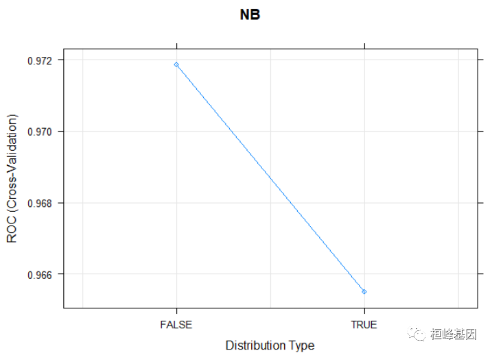
计算混淆矩阵
对于分类模型的只需要看混淆矩阵比较清晰的看出来分类的正确性。
# 6.5. Confusion Matrix Compute the confusion matrix
predProb <- predict(model_BCART, testData, type = "prob")
head(predProb)
##      B    M
## 1 0.00 1.00
## 2 0.28 0.72
## 3 0.48 0.52
## 4 0.00 1.00
## 5 0.00 1.00
## 6 0.00 1.00
predicted = predict(model_BCART, testData)
testData$predProb = predProb$B
testData$diagnosis = as.factor(testData$diagnosis)
confusionMatrix(reference = testData$diagnosis, data = predicted, mode = "everything",
    positive = "B")
## Confusion Matrix and Statistics
##
##           Reference
## Prediction   B   M
##          B 103   7
##          M   4  56
##
##                Accuracy : 0.9353
##                  95% CI : (0.8872, 0.9673)
##     No Information Rate : 0.6294
##     P-Value [Acc > NIR] : <2e-16
##
##                   Kappa : 0.8599
##
##  Mcnemar's Test P-Value : 0.5465
##
##             Sensitivity : 0.9626
##             Specificity : 0.8889
##          Pos Pred Value : 0.9364
##          Neg Pred Value : 0.9333
##               Precision : 0.9364
##                  Recall : 0.9626
##                      F1 : 0.9493
##              Prevalence : 0.6294
##          Detection Rate : 0.6059
##    Detection Prevalence : 0.6471
##       Balanced Accuracy : 0.9258
##
##        'Positive' Class : B
##
绘制ROC曲线
但是根据模型构建后需要进行准确性的评估我们就需要计算一下AUC,绘制ROC曲线来展示一下准确性。
library(ROCR)
pred = prediction(testData$predProb, testData$diagnosis)
perf = performance(pred, measure = "fpr", x.measure = "tpr")
plot(perf, lwd = 2, col = "blue", main = "ROC")
abline(a = 0, b = 1, col = 2, lwd = 1, lty = 2)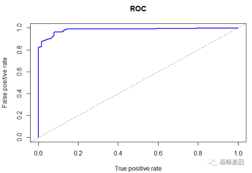
多个分类器比较
# Train the model using rf
model_rf = train(diagnosis ~ ., data = trainData, method = "rf", tuneLength = 2,
    trControl = fitControl)
model_rf
## Random Forest
##
## 398 samples
##  20 predictor
##   2 classes: 'B', 'M'
##
## No pre-processing
## Resampling: Cross-Validated (5 fold)
## Summary of sample sizes: 318, 318, 319, 318, 319
## Resampling results across tuning parameters:
##
##   mtry  ROC        Sens   Spec
##    2    0.9858782  0.976  0.9124138
##   20    0.9792345  0.944  0.9324138
##
## ROC was used to select the optimal model using the largest value.
## The final value used for the model was mtry = 2.
# Train the model using adaboost
model_adaboost = train(diagnosis ~ ., data = trainData, method = "adaboost", tuneLength = 2,
    trControl = fitControl)
model_adaboost
## AdaBoost Classification Trees
##
## 398 samples
##  20 predictor
##   2 classes: 'B', 'M'
##
## No pre-processing
## Resampling: Cross-Validated (5 fold)
## Summary of sample sizes: 319, 318, 318, 318, 319
## Resampling results across tuning parameters:
##
##   nIter  method         ROC        Sens   Spec
##    50    Adaboost.M1    0.9864644  0.984  0.9455172
##    50    Real adaboost  0.8731701  0.992  0.9183908
##   100    Adaboost.M1    0.9909977  0.984  0.9317241
##   100    Real adaboost  0.8495747  0.992  0.9317241
##
## ROC was used to select the optimal model using the largest value.
## The final values used for the model were nIter = 100 and method = Adaboost.M1.
# Train the model using Logitboost
model_LogitBoost = train(diagnosis ~ ., data = trainData, method = "LogitBoost",
    tuneLength = 2, trControl = fitControl)
model_LogitBoost
## Boosted Logistic Regression
##
## 398 samples
##  20 predictor
##   2 classes: 'B', 'M'
##
## No pre-processing
## Resampling: Cross-Validated (5 fold)
## Summary of sample sizes: 319, 318, 318, 318, 319
## Resampling results across tuning parameters:
##
##   nIter  ROC        Sens   Spec
##   11     0.9907517  0.972  0.9462069
##   21     0.9876897  0.976  0.9190805
##
## ROC was used to select the optimal model using the largest value.
## The final value used for the model was nIter = 11.

# Train the model using GBM
model_GBM = train(diagnosis ~ ., data = trainData, method = "gbm", tuneLength = 2,
    trControl = fitControl)
model_GBM
## Stochastic Gradient Boosting
##
## 398 samples
##  20 predictor
##   2 classes: 'B', 'M'
##
## No pre-processing
## Resampling: Cross-Validated (5 fold)
## Summary of sample sizes: 318, 319, 318, 318, 319
## Resampling results across tuning parameters:
##
##   interaction.depth  n.trees  ROC        Sens   Spec
##   1                   50      0.9877770  0.964  0.8988506
##   1                  100      0.9890437  0.980  0.9121839
##   2                   50      0.9900460  0.968  0.9259770
##   2                  100      0.9897609  0.976  0.9393103
##
## Tuning parameter 'shrinkage' was held constant at a value of 0.1
##
## Tuning parameter 'n.minobsinnode' was held constant at a value of 10
## ROC was used to select the optimal model using the largest value.
## The final values used for the model were n.trees = 50, interaction.depth =
##  2, shrinkage = 0.1 and n.minobsinnode = 10.

# Train the model using PAM
model_PAM = train(diagnosis ~ ., data = trainData, method = "pam", tuneLength = 2,
    trControl = fitControl)
## 123456789101112131415161718192021222324252627282930111111
model_PAM
## Nearest Shrunken Centroids
##
## 398 samples
##  20 predictor
##   2 classes: 'B', 'M'
##
## No pre-processing
## Resampling: Cross-Validated (5 fold)
## Summary of sample sizes: 318, 318, 318, 319, 319
## Resampling results across tuning parameters:
##
##   threshold   ROC     Sens  Spec
##    0.3730189  0.9536  0.94  0.8048276
##   10.4445296  0.5000  1.00  0.0000000
##
## ROC was used to select the optimal model using the largest value.
## The final value used for the model was threshold = 0.3730189.

# Train the model using NB
model_NB = train(diagnosis ~ ., data = trainData, method = "naive_bayes", tuneLength = 2,
    trControl = fitControl)
model_NB
## Naive Bayes
##
## 398 samples
##  20 predictor
##   2 classes: 'B', 'M'
##
## No pre-processing
## Resampling: Cross-Validated (5 fold)
## Summary of sample sizes: 319, 319, 318, 318, 318
## Resampling results across tuning parameters:
##
##   usekernel  ROC        Sens   Spec
##   FALSE      0.9693701  0.936  0.9124138
##    TRUE      0.9695218  0.908  0.8926437
##
## Tuning parameter 'laplace' was held constant at a value of 0
## Tuning
##  parameter 'adjust' was held constant at a value of 1
## ROC was used to select the optimal model using the largest value.
## The final values used for the model were laplace = 0, usekernel = TRUE
##  and adjust = 1.

# Train the model using NNNET
model_NNET = train(diagnosis ~ ., data = trainData, method = "nnet", tuneLength = 2,
    trControl = fitControl)
model_NNET
## Neural Network
##
## 398 samples
##  20 predictor
##   2 classes: 'B', 'M'
##
## No pre-processing
## Resampling: Cross-Validated (5 fold)
## Summary of sample sizes: 318, 318, 319, 318, 319
## Resampling results across tuning parameters:
##
##   size  decay  ROC        Sens   Spec
##   1     0.0    0.9628506  0.988  0.9326437
##   1     0.1    0.9798529  0.968  0.9257471
##   3     0.0    0.9658184  0.964  0.8983908
##   3     0.1    0.9871034  0.972  0.9459770
##
## ROC was used to select the optimal model using the largest value.
## The final values used for the model were size = 3 and decay = 0.1.

models_compare <- resamples(list(ADABOOST = model_adaboost, RF = model_rf, LOGITBOOST = model_LogitBoost,
    GBM = model_GBM, PAM = model_PAM, NB = model_NB, NNET = model_NNET, BaggedCART = model_BCART))
summary(models_compare)
##
## Call:
## summary.resamples(object = models_compare)
##
## Models: ADABOOST, RF, LOGITBOOST, GBM, PAM, NB, NNET, BaggedCART
## Number of resamples: 5
##
## ROC
##                 Min.   1st Qu.    Median      Mean   3rd Qu.      Max. NA's
## ADABOOST   0.9848276 0.9848276 0.9900000 0.9909977 0.9953333 1.0000000    0
## RF         0.9517241 0.9850000 0.9953333 0.9858782 0.9973333 1.0000000    0
## LOGITBOOST 0.9783333 0.9862069 0.9926667 0.9907517 0.9965517 1.0000000    0
## GBM        0.9653333 0.9868966 0.9980000 0.9900460 1.0000000 1.0000000    0
## PAM        0.9046667 0.9306667 0.9703448 0.9536000 0.9726667 0.9896552    0
## NB         0.9440000 0.9682759 0.9773333 0.9695218 0.9780000 0.9800000    0
## NNET       0.9751724 0.9820000 0.9903448 0.9871034 0.9906667 0.9973333    0
## BaggedCART 0.9583333 0.9872414 0.9886207 0.9847057 0.9900000 0.9993333    0
##
## Sens
##            Min. 1st Qu. Median  Mean 3rd Qu. Max. NA's
## ADABOOST   0.96    0.98   0.98 0.984    1.00 1.00    0
## RF         0.96    0.96   0.98 0.976    0.98 1.00    0
## LOGITBOOST 0.94    0.96   0.96 0.972    1.00 1.00    0
## GBM        0.94    0.94   0.96 0.968    1.00 1.00    0
## PAM        0.90    0.94   0.94 0.940    0.96 0.96    0
## NB         0.88    0.88   0.88 0.908    0.92 0.98    0
## NNET       0.92    0.96   0.98 0.972    1.00 1.00    0
## BaggedCART 0.90    0.92   0.94 0.936    0.94 0.98    0
##
## Spec
##                 Min.   1st Qu.    Median      Mean   3rd Qu.      Max. NA's
## ADABOOST   0.8275862 0.9310345 0.9333333 0.9317241 0.9666667 1.0000000    0
## RF         0.8333333 0.8620690 0.9000000 0.9124138 0.9666667 1.0000000    0
## LOGITBOOST 0.8333333 0.9310345 0.9666667 0.9462069 1.0000000 1.0000000    0
## GBM        0.8333333 0.8965517 0.9000000 0.9259770 1.0000000 1.0000000    0
## PAM        0.7333333 0.7333333 0.8275862 0.8048276 0.8333333 0.8965517    0
## NB         0.7333333 0.8666667 0.9310345 0.8926437 0.9655172 0.9666667    0
## NNET       0.9310345 0.9333333 0.9333333 0.9459770 0.9655172 0.9666667    0
## BaggedCART 0.8666667 0.8965517 0.9310345 0.9321839 0.9666667 1.0000000    0
# Draw box plots to compare models
scales <- list(x = list(relation = "free"), y = list(relation = "free"))
bwplot(models_compare, scales = scales)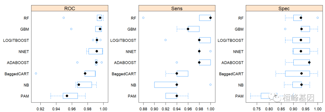
生成测试集结果
绘制 Calibration Curves
## Generate the test set results
results <- data.frame(Diagnosis = testData$diagnosis)
results$RF <- predict(model_rf, testData, type = "prob")[, "B"]
results$adaboost <- predict(model_adaboost, testData, type = "prob")[, "B"]
results$LogitBoost <- predict(model_LogitBoost, testData, type = "prob")[, "B"]
results$GBM <- predict(model_GBM, testData, type = "prob")[, "B"]
results$PAM <- predict(model_PAM, testData, type = "prob")[, "B"]
results$NB <- predict(model_NB, testData, type = "prob")[, "B"]
results$NNET <- predict(model_NNET, testData, type = "prob")[, "B"]
results$BaggedCART <- predict(model_BCART, testData, type = "prob")[, "B"]
head(results)
##   Diagnosis    RF   adaboost   LogitBoost        GBM          PAM           NB
## 1         M 0.008 0.03767170 0.0066928509 0.01809233 1.538730e-02 4.991767e-14
## 2         M 0.232 0.23080168 0.0474258732 0.08444066 6.673408e-05 5.224971e-07
## 3         M 0.786 0.73120191 0.7310585786 0.58123387 9.392887e-01 9.999959e-01
## 4         M 0.038 0.06663126 0.0009110512 0.01792707 1.155797e-01 4.615765e-09
## 5         M 0.190 0.23191784 0.0066928509 0.02085581 4.748940e-03 9.490869e-13
## 6         M 0.062 0.16372403 0.0474258732 0.05115349 9.553552e-03 1.255993e-11
##           NNET BaggedCART
## 1 0.0002086345       0.00
## 2 0.0214382430       0.28
## 3 0.1396975039       0.48
## 4 0.0013018679       0.00
## 5 0.8918220960       0.00
## 6 0.0003457715       0.00
trellis.par.set(caretTheme())
cal_obj <- calibration(Diagnosis ~ RF + adaboost + LogitBoost + GBM + PAM + NB +
    NNET + BaggedCART, data = results, cuts = 13)
plot(cal_obj, type = "l", auto.key = list(columns = 8, lines = TRUE, points = FALSE))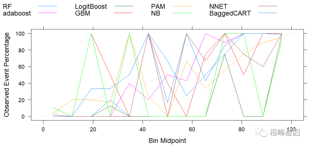
还有一种ggplot方法可以显示子集内部比例的置信区间:
ggplot(cal_obj)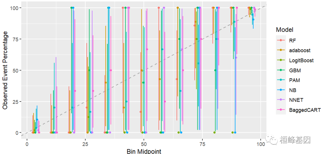
号外号外,桓峰基因单细胞生信分析免费培训课程即将开始快来报名吧!
桓峰基因,铸造成功的您!
未来桓峰基因公众号将不间断的推出单细胞系列生信分析教程,
敬请期待!!
桓峰基因官网正式上线,请大家多多关注,还有很多不足之处,大家多多指正!http://www.kyohogene.com/
桓峰基因和投必得合作,文章润色优惠85折,需要文章润色的老师可以直接到网站输入领取桓峰基因专属优惠券码:KYOHOGENE,然后上传,付款时选择桓峰基因优惠券即可享受85折优惠哦!https://www.topeditsci.com/


 4109
4109

 被折叠的 条评论
为什么被折叠?
被折叠的 条评论
为什么被折叠?
 到【灌水乐园】发言


