MachineLearning 38. 机器学习之基于最近收缩质心分类法的肿瘤亚型分类器 (pamr)

最新推荐文章于 2024-06-18 17:30:32 发布

桓峰基因

最新推荐文章于 2024-06-18 17:30:32 发布

阅读量703

点赞数 14

文章标签：机器学习人工智能

本文链接：https://blog.csdn.net/weixin_41368414/article/details/139513134

版权

简介

基于最近收缩质心分类法(nearest shrunken centroids)的基因表达谱预测癌症类别的方法。缩小了原型，从而得到了一个通常比竞争方法更准确的分类器。“最近的收缩质心”方法确定了最能表征每个类别的基因子集。该技术是通用的，可用于许多其他分类问题。为了证明其有效性，表明该方法在寻找用于分类小圆蓝细胞肿瘤和白血病的基因方面非常有效。

软件包安装

软件包安装：

install.packages('pamr')

数据读取

khan 有2309行和65列。这些是Tibshirani等人在PNAS上发表的关于最近的收缩质心的论文中使用的数据集之一。第一行包含示例标签。前两列是基因id和名称。

读取数据并构造输入列表，包括

x：表达矩阵
y：类型
geneid：基因名
genename：基因名称

library(pamr)
data(khan)
dim(khan)
## [1] 2309   65

khan[1:5, 1:5]
##       X                         X1      sample1      sample2      sample3
## 1                                           EWS          EWS          EWS
## 2 GENE1  "\\"catenin (cadherin-a"   0.773343723 -0.078177781 -0.084469157
## 3 GENE2   "farnesyl-diphosphate"   -2.438404816 -2.415753791 -1.649739209
## 4 GENE3  "\\"phosphofructokinase"  -0.482562158  0.412771683 -0.241307522
## 5 GENE4   "cytochrome c-1"         -2.721135441 -2.825145973  -2.87528612

colnames(khan)
##  [1] "X"        "X1"       "sample1"  "sample2"  "sample3"  "sample4" 
##  [7] "sample5"  "sample6"  "sample7"  "sample8"  "sample9"  "sample10"
## [13] "sample11" "sample12" "sample13" "sample14" "sample15" "sample16"
## [19] "sample17" "sample18" "sample19" "sample20" "sample21" "sample22"
## [25] "sample23" "sample24" "sample25" "sample26" "sample27" "sample28"
## [31] "sample29" "sample30" "sample31" "sample32" "sample33" "sample34"
## [37] "sample35" "sample36" "sample37" "sample38" "sample39" "sample40"
## [43] "sample41" "sample42" "sample43" "sample44" "sample45" "sample46"
## [49] "sample47" "sample48" "sample49" "sample50" "sample51" "sample52"
## [55] "sample53" "sample54" "sample55" "sample56" "sample57" "sample58"
## [61] "sample59" "sample60" "sample61" "sample62" "sample63"

x <- data.matrix(khan[-1, c(-1, -2)])
x[1:5, 1:5]
##   sample1 sample2 sample3 sample4 sample5
## 2    1873      57      53    2059    1537
## 3    1251    1350    1140    1385    1261
## 4     314    1758     162    1857    1939
## 5    1324    1428    1468    1250    1666
## 6     776     476     679     772    1307

rownames(x) = khan[-1, 1]
y <- as.vector(t(khan[1, c(-1, -2)]))
is.vector(y)
## [1] TRUE

length(y)
## [1] 63

mydata <- list(x = x, y = factor(y), geneid = rownames(x), genenames = paste(khan[-1,
    1], khan[-1, 2], " "))

实例操作

参数说明

Arguments

data： The input data. A list with components: x- an expression genes in the rows, samples in the columns), and y- a vector of the class labels for each sample. Optional components- genenames, a vector of gene names, and geneid- a vector of gene identifiers.
gene.subset Subset of genes to be used. Can be either a logical vector of length total number of genes, or a list of integers of the row numbers of the genes to be used
sample.subset Subset of samples to be used. Can be either a logical vector of length total number of samples, or a list of integers of the column numbers of the samples to be used.
threshold A vector of threshold values for the centroid shrinkage.Default is a set of 30 values chosen by the software
n.threshold Number of threshold values desired (default 30)
scale.sd Scale each threshold by the wthin class standard deviations? Default: true
threshold.scale Additional scaling factors to be applied to the thresholds. Vector of length equal to the number of classes. Default- a vectors of ones.
se.scale Vector of scaling factors for the within class standard errors. Default is sqrt(1/n.class-1/n), where n is the overall sample size and n.class is the sample sizes in each class. This default adjusts for different class sizes.
offset.percent Fudge factor added to the denominator of each t-statistic, expressed as a percentile of the gene standard deviation values. This is a small positive quantity to penalize genes with expression values near zero, which can result in very large ratios. This factor is expecially impotant for Affy data. Default is the median of the standard deviations of each gene.
hetero Should a heterogeneity transformation be done? If yes, hetero must be set to one of the class labels (see Details below). Default is no (hetero=NULL)
prior Vector of length the number of classes, representing prior probabilities for each of the classes. The prior is used in Bayes rule for making class prediction. Default is NULL, and prior is then taken to be n.class/n, where n is the overall sample size and n.class is the sample sizes in each class.
remove.zeros Remove threshold values yielding zero genes? Default TRUE
sign.contrast Directions of allowed deviations of class-wise average gene expression from the overall average gene expression. Default is “both” (positive or negative). Can also be set to “positive” or “negative”.
ngroup.survival Number of groups formed for survival data. Default 2

构建模型

训练分类器（非生存数据）

# train classifier
mytrain <- pamr.train(mydata, gene.subset = NULL, sample.subset = NULL, threshold = NULL,
    n.threshold = 30, scale.sd = TRUE, threshold.scale = NULL, se.scale = NULL, offset.percent = 50,
    hetero = NULL, prior = NULL, remove.zeros = TRUE, sign.contrast = "both", ngroup.survival = 4)
## 123456789101112131415161718192021222324252627282930

交叉验证

通过交叉验证我们可以根据errors最低，筛选基因threshold，确定基因个数：当errors=0,threshold=1.821,筛选基因数为243个。

mycv <- pamr.cv(mytrain, mydata)
## 1234Fold 1 :123456789101112131415161718192021222324252627282930
## Fold 2 :123456789101112131415161718192021222324252627282930
## Fold 3 :123456789101112131415161718192021222324252627282930
## Fold 4 :123456789101112131415161718192021222324252627282930
## Fold 5 :123456789101112131415161718192021222324252627282930
## Fold 6 :123456789101112131415161718192021222324252627282930
## Fold 7 :123456789101112131415161718192021222324252627282930
## Fold 8 :123456789101112131415161718192021222324252627282930

mycv
## Call:
## pamr.cv(fit = mytrain, data = mydata)
##    threshold nonzero errors
## 1  0.000     2308    3     
## 2  0.202     2264    4     
## 3  0.405     2133    4     
## 4  0.607     1834    5     
## 5  0.809     1469    4     
## 6  1.012     1115    5     
## 7  1.214      790    5     
## 8  1.416      537    4     
## 9  1.619      362    3     
## 10 1.821      243    1     
## 11 2.023      159    0     
## 12 2.226      102    2     
## 13 2.428       72    3     
## 14 2.630       56    3     
## 15 2.832       38    5     
## 16 3.035       24    11    
## 17 3.237       17    17    
## 18 3.439       15    22    
## 19 3.642        9    23    
## 20 3.844        5    23    
## 21 4.046        4    23    
## 22 4.249        4    24    
## 23 4.451        4    25    
## 24 4.653        3    25    
## 25 4.856        3    28    
## 26 5.058        3    33    
## 27 5.260        1    34    
## 28 5.463        1    40    
## 29 5.665        1    40    
## 30 5.867        0    40

pamr.plotcv(mycv)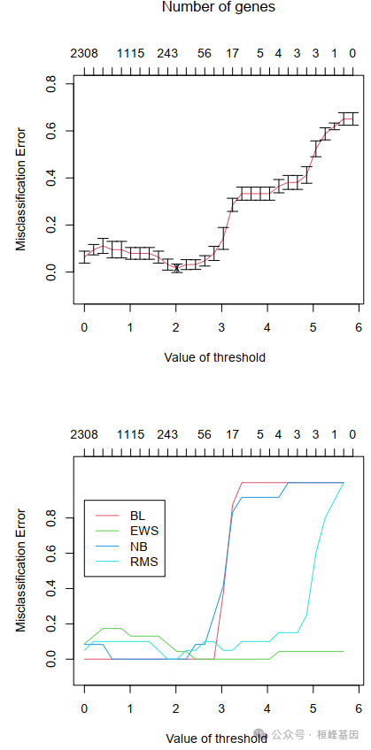

pamr.plotcvprob(mycv, mydata, threshold = 2)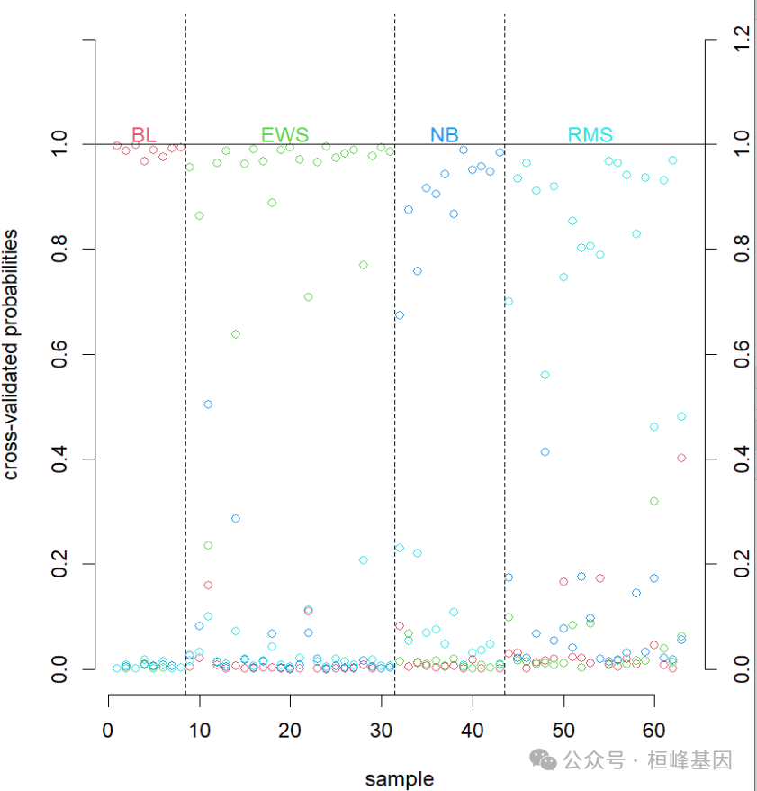

pamr.listgenes(mytrain, mydata, threshold = 3.5)[1:10, ]
##       id       BL-score EWS-score NB-score RMS-score
##  [1,] GENE1954 0        0.3933    0        0        
##  [2,] GENE1955 0        0         0        0.2979   
##  [3,] GENE1389 0        0.2687    0        0        
##  [4,] GENE246  0        0.1916    0        0        
##  [5,] GENE842  0        0         -0.0784  0        
##  [6,] GENE545  0        0.061     0        0        
##  [7,] GENE742  0        0         0.0549   0        
##  [8,] GENE951  -0.0507  0         0        0        
##  [9,] GENE84   -0.0416  0         0        0        
## [10,] GENE910  0        0         0        0.0243   
## [11,] GENE1645 0        0.0239    0        0        
## [12,] GENE77   -0.0149  0         0        0        
## [13,] GENE509  0        0         0        0.0089   
## [14,] GENE1772 0        0.0067    0        0
##       id         BL-score  EWS-score NB-score  RMS-score
##  [1,] "GENE1954" "0"       "0.3933"  "0"       "0"      
##  [2,] "GENE1955" "0"       "0"       "0"       "0.2979" 
##  [3,] "GENE1389" "0"       "0.2687"  "0"       "0"      
##  [4,] "GENE246"  "0"       "0.1916"  "0"       "0"      
##  [5,] "GENE842"  "0"       "0"       "-0.0784" "0"      
##  [6,] "GENE545"  "0"       "0.061"   "0"       "0"      
##  [7,] "GENE742"  "0"       "0"       "0.0549"  "0"      
##  [8,] "GENE951"  "-0.0507" "0"       "0"       "0"      
##  [9,] "GENE84"   "-0.0416" "0"       "0"       "0"      
## [10,] "GENE910"  "0"       "0"       "0"       "0.0243"

基因筛选

绘制筛选结果时发现，数量太多，我们可以减少点基因数据，控制threshold作图：

pamr.geneplot(mytrain, mydata, threshold = 3.5)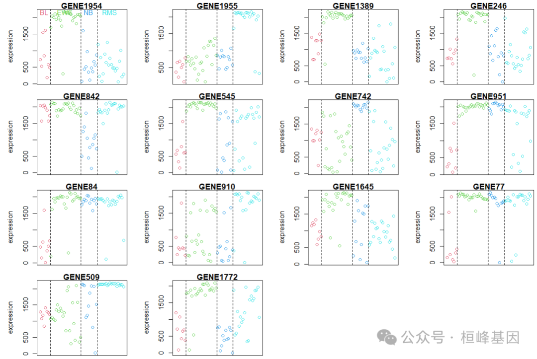

pamr.plotcen(mytrain, mydata, threshold = 3.5)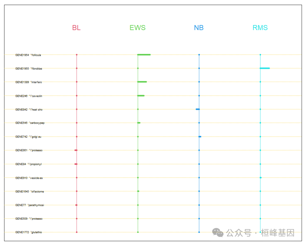

一致性分析

pamr软件包提供交叉验证的函数 pamr.confusion，我们可以看下当threshold=3.5时的准确性：

pamr.confusion(mytrain, threshold = 3.5)
##     BL EWS NB RMS Class Error rate
## BL   0   4  0   4             1.00
## EWS  0  23  0   0             0.00
## NB   0   1  0  11             1.00
## RMS  0   1  0  19             0.05
## Overall error rate= 0.323

pamr.confusion(mycv, threshold = 3.5)
##     BL EWS NB RMS Class Error rate
## BL   0   4  0   4       1.00000000
## EWS  0  22  0   1       0.04347826
## NB   0   1  0  11       1.00000000
## RMS  0   2  0  18       0.10000000
## Overall error rate= 0.353

prob <- pamr.predict(mytrain, mydata$x, threshold = 1, type = "posterior")
pamr.indeterminate(prob, mingap = 0.75)
##  [1] EWS  EWS  EWS  EWS  EWS  <NA> EWS  EWS  EWS  EWS  EWS  EWS  EWS  EWS  EWS  EWS  EWS  EWS  EWS  EWS  EWS  EWS  EWS  RMS  RMS  RMS  RMS  RMS  RMS  RMS  RMS  RMS  RMS  RMS  RMS  RMS  RMS  RMS  RMS  RMS  RMS  RMS  RMS  NB   NB   NB   NB   NB   NB   NB   NB   NB   NB   NB   NB   BL   BL   BL   BL   BL   BL   BL   BL  
## Levels: BL EWS NB RMS

训练分类器（生存数据）

我们仍然使用khan数据，通过模型生存数据，将添加time 和 status,进行生存分析：

gendata <- function(n = 100, p = 2000) {
    tim <- 3 * abs(rnorm(n))
    u <- runif(n, min(tim), max(tim))
    y <- pmin(tim, u)
    ic <- 1 * (tim < u)
    m <- median(tim)
    x <- matrix(rnorm(p * n), ncol = n)
    x[1:100, tim > m] <- x[1:100, tim > m] + 3
    return(list(x = x, y = y, ic = ic))
}
junk <- gendata(n = 63)
mydata$time = junk$y
mydata$status = junk$ic
a3 <- pamr.train(mydata, ngroup.survival = 4)
## 123456789101112131415161718192021222324252627282930

a3
## Call:
## pamr.train(data = mydata, ngroup.survival = 4)
##    threshold nonzero errors
## 1  0.000     2308    0     
## 2  0.202     2264    0     
## 3  0.405     2133    0     
## 4  0.607     1834    0     
## 5  0.809     1469    0     
## 6  1.012     1115    0     
## 7  1.214      790    0     
## 8  1.416      537    0     
## 9  1.619      362    0     
## 10 1.821      243    0     
## 11 2.023      159    0     
## 12 2.226      102    0     
## 13 2.428       72    0     
## 14 2.630       56    0     
## 15 2.832       38    2     
## 16 3.035       24    6     
## 17 3.237       17    16    
## 18 3.439       15    21    
## 19 3.642        9    21    
## 20 3.844        5    21    
## 21 4.046        4    21    
## 22 4.249        4    21    
## 23 4.451        4    22    
## 24 4.653        3    22    
## 25 4.856        3    25    
## 26 5.058        3    34    
## 27 5.260        1    40    
## 28 5.463        1    40    
## 29 5.665        1    40    
## 30 5.867        0    40

根据计算预测结果，并进行绘制生存曲线：

yhat <- pamr.predict(a3, mydata$x, threshold = 1)
proby <- pamr.surv.to.class2(mydata$time, mydata$status, n.class = a3$ngroup.survival)$prob
pamr.test.errors.surv.compute(proby, yhat)
## $confusion
##           1         2        3        4 Class Error rate
## 1 2.0000000  3.338030 2.040816 4.100078        0.8257677
## 2 3.1766702  2.394302 2.210077 3.502929        0.7878140
## 3 0.6362316  4.371070 2.566928 6.466078        0.8171744
## 4 2.1870982 12.896598 5.182178 5.930915        0.7736014
## 
## $error
## [1] 0.7568664

pamr.plotsurvival(yhat, mydata$time, mydata$status)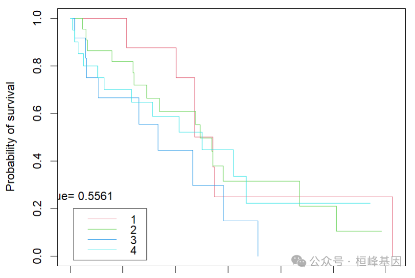

绘制ROC曲线

由于我们所作的模型根时间密切相关因此我们选择timeROC,可以快速的技术出来不同时期的ROC，进一步作图：

library(timeROC)
res <- timeROC(T = mydata$time, delta = mydata$status, marker = proby[, 1], cause = 1, weighting = "marginal", times = c(1, 2, 3), ROC = TRUE, iid = TRUE)
res$AUC
##       t=1       t=2       t=3 
## 0.8617985 0.6870657 0.6220219

confint(res, level = 0.95)$CI_AUC
##      2.5% 97.5%
## t=1 74.65 97.70
## t=2 59.69 77.72
## t=3 55.75 68.65

plot(res, time = 1, col = "red", title = FALSE, lwd = 2)
plot(res, time = 2, add = TRUE, col = "blue", lwd = 2)
plot(res, time = 3, add = TRUE, col = "green", lwd = 2)
legend("bottomright", c(paste("1 Years ", round(res$AUC[1], 2)), paste("2 Years ", round(res$AUC[2], 2)), paste("3 Years ", round(res$AUC[3], 2))), col = c("red", "blue", "green"), lty = 1, lwd = 2)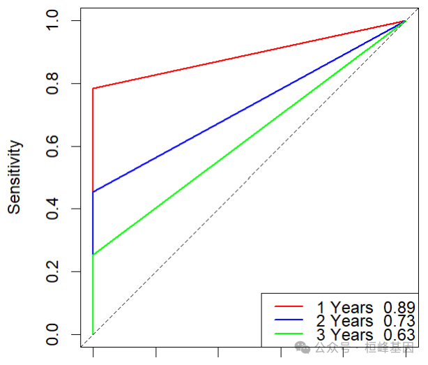

不同时间节点的AUC曲线及其置信区间

再分析不同时间节点的AUC曲线及其置信区间，由于数据量非常小，此图并不明显。

plotAUCcurve(res, conf.int = TRUE, col = "red")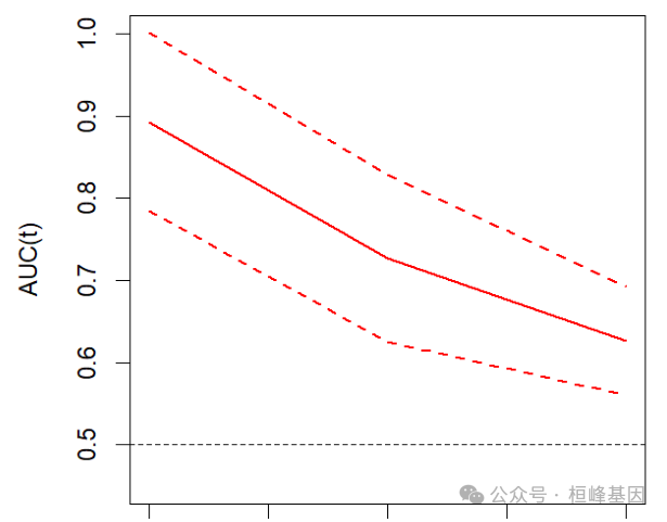

Reference

Robert Tibshirani, Trevor Hastie, Balasubramanian Narasimhan, and Gilbert Chu Diagnosis of multiple cancer types by shrunken centroids of gene expression PNAS 99: 6567-6572. Available at www.pnas.org
Khan, J., Wei, J., Ringnér, M. et al. Classification and diagnostic prediction of cancers using gene expression profiling and artificial neural networks. Nat Med 7, 673–679 (2001). https://doi.org/10.1038/89044

基于机器学习构建临床预测模型

MachineLearning 1. 主成分分析（PCA）

MachineLearning 2. 因子分析（Factor Analysis）

MachineLearning 3. 聚类分析（Cluster Analysis）

MachineLearning 4. 癌症诊断方法之 K-邻近算法（KNN）

MachineLearning 5. 癌症诊断和分子分型方法之支持向量机（SVM)

MachineLearning 6. 癌症诊断机器学习之分类树（Classification Trees)

MachineLearning 7. 癌症诊断机器学习之回归树（Regression Trees)

MachineLearning 8. 癌症诊断机器学习之随机森林（Random Forest)

MachineLearning 9. 癌症诊断机器学习之梯度提升算法（Gradient Boosting)

MachineLearning 10. 癌症诊断机器学习之神经网络（Neural network)

MachineLearning 11. 机器学习之随机森林生存分析（randomForestSRC）

MachineLearning 12. 机器学习之降维方法t-SNE及可视化(Rtsne)

MachineLearning 13. 机器学习之降维方法UMAP及可视化 (umap)

MachineLearning 14. 机器学习之集成分类器(AdaBoost)

MachineLearning 15. 机器学习之集成分类器(LogitBoost)

MachineLearning 16. 机器学习之梯度提升机(GBM)

MachineLearning 17. 机器学习之围绕中心点划分算法(PAM)

MachineLearning 18. 机器学习之贝叶斯分析类器(Naive Bayes)

MachineLearning 19. 机器学习之神经网络分类器(NNET)

MachineLearning 20. 机器学习之袋装分类回归树(Bagged CART)

MachineLearning 21. 机器学习之临床医学上的生存分析(xgboost)

MachineLearning 22. 机器学习之有监督主成分分析筛选基因(SuperPC)

MachineLearning 23. 机器学习之岭回归预测基因型和表型(Ridge)

MachineLearning 24. 机器学习之似然增强Cox比例风险模型筛选变量及预后估计(CoxBoost)

MachineLearning 25. 机器学习之支持向量机应用于生存分析(survivalsvm)

MachineLearning 26. 机器学习之弹性网络算法应用于生存分析(Enet)

MachineLearning 27. 机器学习之逐步Cox回归筛选变量(StepCox)

MachineLearning 28. 机器学习之偏最小二乘回归应用于生存分析(plsRcox)

MachineLearning 29. 机器学习之嵌套交叉验证(Nested CV)

MachineLearning 30. 机器学习之特征选择森林之神(Boruta)

MachineLearning 31. 机器学习之基于RNA-seq的基因特征筛选 (GeneSelectR)

MachineLearning 32. 机器学习之支持向量机递归特征消除的特征筛选 (mSVM-RFE)

MachineLearning 33. 机器学习之时间-事件预测与神经网络和Cox回归

MachineLearning 34. 机器学习之竞争风险生存分析的深度学习方法(DeepHit)

MachineLearning 35. 机器学习之Lasso+Cox回归筛选变量 (LassoCox)

MachineLearning 36. 机器学习之基于神经网络的Cox比例风险模型 (Deepsurv)

桓峰基因，铸造成功的您！

未来桓峰基因公众号将不间断的推出单细胞系列生信分析教程，

敬请期待！！

桓峰基因官网正式上线，请大家多多关注，还有很多不足之处，大家多多指正！http://www.kyohogene.com/

桓峰基因和投必得合作，文章润色优惠85折，需要文章润色的老师可以直接到网站输入领取桓峰基因专属优惠券码：KYOHOGENE，然后上传，付款时选择桓峰基因优惠券即可享受85折优惠哦！https://www.topeditsci.com/

桓峰基因

关注

14
点赞
踩
29

收藏

觉得还不错? 一键收藏
0
评论
MachineLearning 38. 机器学习之基于最近收缩质心分类法的肿瘤亚型分类器 (pamr)

简介基于最近收缩质心分类法(nearest shrunken centroids)的基因表达谱预测癌症类别的方法。缩小了原型，从而得到了一个通常比竞争方法更准确的分类器。“最近的收缩质心”方法确定了最能表征每个类别的基因子集。该技术是通用的，可用于许多其他分类问题。为了证明其有效性，表明该方法在寻找用于分类小圆蓝细胞肿瘤和白血病的基因方面非常有效。软件包安装软件包安装：install.p...
复制链接

扫一扫