手把手教做无人驾驶算法（二十七）--关于MPC扰动不变集的分析

 Disturbance invariant set

I think one may get stuck at computation of what paper [1] called "disturbance invariant set". The disturbance invariant set is an infinite Minkowski addition Z = W ⨁ Ak*W ⨁ Ak^2*W..., where ⨁ denotes Minkowski addition. Obtaining this analytically is impossible, and then, what comes ones' mind first may be an approximation of that by truncation: Z_approx = W ⨁ Ak*W...⨁ Ak^n*W. This approximation, however, leads to Z_approx ⊂ Z, which means Z_approx is not disturbance invariant. So, we must multiply it by some parameter alpha and get Z_approx = alpha*(W ⨁ Ak*W...⨁ Ak^n*W) so that Z ⊂ Z_approx is guaranteed. (see example/DisturbanceLinearSystem.m for this implementation). The order of truncation and alpha are tuning parameters, and I chose values that are large enough. But, if you want to choose them in a more sophisticated way, paper [3] will be useful. Also, example/example_dist_inv_set.m may help you understand how disturbance the invariant set works.

主函数（example_dist_inv_set.m）：

function test
% addpath('../src/')
% addpath('../src/utils/')

% specify your own discrete linear system
A = [1 1; 0 1];
B = [0.5; 1]; 
Q = diag([1, 1]);
R = 0.1;

% construct a convex set of system noise (2dim here)
W_vertex = [0.15, 0.85; 0.15, -0.85; -0.15, -0.15; -0.15, 0.15];
W = Polyhedron(W_vertex);

% construct disturbance Linear system
% note that disturbance invariant set Z is computed and stored as member variable in the constructor.
disturbance_system = DisturbanceLinearSystem(A, B, Q, R, W); 
[K_tmp, obj.P] = dlqr(A, B, Q, R)
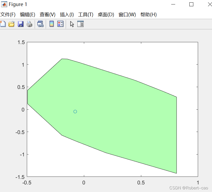
% you can see that with any disturbance bounded by W, the state is guaranteed to inside Z
x = zeros(2); % initial state 
for i = 1:50
    u = -K_tmp * (x - 0);
    x = disturbance_system.propagate(x, u); % disturbance is considered inside the method
    clf;
    Graphics.show_convex(disturbance_system.Z, 'g', 'FaceAlpha', .3); % show Z
    scatter(x(1, :), x(2, :)); % show particle
    pause(0.01);
end
end

调用函数（DisturbanceLinearSystem.m）：

classdef DisturbanceLinearSystem < handle

    properties (SetAccess = private)
        W % convex set of distrubance
        Z % disturbance invariant set
        
        % common notation for linear system
        A; B; % dynamics x[k+1] = A*x[k]+B*u[k]
        nx; nu; % dim of state space and input space
        Q; R; % quadratic stage cost for LQR
        K; % LQR feedback coefficient vector: u=Kx
        P; % optimal cost function of LQR is x'*P*x
        Ak %: A + BK closed loop dynamics
        
    end

    methods (Access = public)

        function obj = DisturbanceLinearSystem(A, B, Q, R, W)
%             obj = obj@LinearSystem(A, B, Q, R);
            obj.A = A;
            obj.B = B;
            obj.Q = Q;
            obj.R = R;
            obj.nx = size(A, 1);
            obj.nu = size(B, 2);

            [K_tmp, obj.P] = dlqr(obj.A, obj.B, obj.Q, obj.R);
            obj.K = -K_tmp;
            obj.Ak = (obj.A+obj.B*obj.K);
            obj.W = W;
            obj.Z = obj.compute_mrpi_set(1e-4);
        end

        function x_new = propagate(obj, x, u)
            w = obj.pick_random_disturbance();
            x_new = obj.A * x + obj.B * u + w;
        end

    end

    methods (Access = public)

        function w = pick_random_disturbance(obj)
            % pick disturbance form uniform distribution
            verts = obj.W.V;
            b_max = max(verts)';
            b_min = min(verts)';

            % generate random until it will be inside of W
            while true
                w = rand(obj.nx, 1) .* (b_max - b_min) + b_min; 
                if obj.W.contains(w)
                    break
                end
            end
        end

        function Fs = compute_mrpi_set(obj, epsilon)
            % Computes an invariant approximation of the minimal robust positively
            % invariant set for 
            % x^{+} = Ax + w with w \in W
            % according to Algorithm 1 in 'Invariant approximations of
            % the minimal robust positively invariant set' by Rakovic et al. 
            % Requires a matrix A, a Polytope W, and a tolerance 'epsilon'.  
            [nx,~] = size(obj.Ak); 
            s = 0; 
            alpha = 1000;
            Ms = 1000;
            E = eye(nx);
            it = 0;
            while(alpha > epsilon/(epsilon + Ms))
                s = s+1;
                alpha = max(obj.W.support(obj.Ak^s*(obj.W.A)')./obj.W.b);
                mss = zeros(2*nx,1);
                for i = 1:s
                    mss = mss+obj.W.support([obj.Ak^i, -obj.Ak^i]);
                end
                Ms = max(mss);
                it = it+1;
            end

            Fs = obj.W;
            for i =1:s-1
                Fs = Fs+obj.Ak^i*obj.W;
            end
            Fs = (1/(1-alpha))*Fs;
        end
        
        
        

    end
end

结果：

参考资料：

[1] Langson, Wilbur, et al. "Robust model predictive control using tubes." Automatica 40.1 (2004): 125-133.

[2] Mayne, David Q., María M. Seron, and S. V. Raković. "Robust model predictive control of constrained linear systems with bounded disturbances." Automatica 41.2 (2005): 219-224.

[3] Rakovic, Sasa V., et al. "Invariant approximations of the minimal robust positively invariant set." IEEE Transactions on Automatic Control 50.3 (2005): 406-410.

GitHub - HiroIshida/robust-tube-mpc: Robust model predictive control using tube