Haar小波下采样模块

夏天是冰红茶

已于 2024-12-31 17:41:37 修改

阅读量1w

点赞数 36

分类专栏： pytorch复现文章标签：深度学习机器学习人工智能

于 2024-01-22 23:08:52 首次发布

本文链接：https://blog.csdn.net/m0_62919535/article/details/135758371

版权

pytorch复现专栏收录该内容

22 篇文章

订阅专栏

论文原址：Haar wavelet downsampling: A simple but effective downsampling module for semantic segmentation - ScienceDirect

原文代码：HWD/HWD.py at main · apple1986/HWD (github.com)

介绍

深度卷积神经网络（DCNN）通常采用标准的下采样操作，例如最大池化、平均池化和跨步卷积，这可能会导致信息丢失。丢失的信息，如边界和纹理，对于语义分割可能是必不可少的。为了缓解这个问题，一般有下面四种方法：

通过跳过连接到解码器子网（如U-Net、LCU-Net、CENet、LinkNet和RefineNet ）。
提取具有空间金字塔池化或扩展卷积的多尺度特征图到融合模块中（如DeepLab、PSPNet、PCPLP-Net、BiSenet和ICNet）。
向编码器提供多模态图像（如DiSegNet、MMADT、CANet和CCFFNet）。
增加先验信息。轮廓增强关注模块，旨在从CT图像中提取边界和形状线索，以细化分割区域。

这些方法的主要目的是通过基于多尺度、先验指导、多模态等各种策略提供更多的学习信息或特征，帮助下采样特征与分割标签之间建立良好的关系。

因此，是否可以设计一个保留信息的下采样模块，使DCNNs中尽可能多地保留信息进行语义分割?这就是作者的想法。

下采样模块

最大池化与平均池化

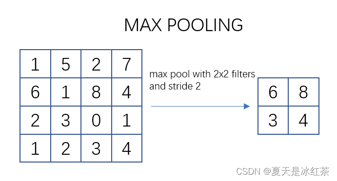
池化过程类似于卷积过程。在这个示意图中，我们看到对一个 4x4 的特征图邻域进行操作，使用了一个 2x2 的滤波器，步长为2进行扫描。这个过程被称为最大池化（Max Pooling），其中选择邻域内的最大值并输出到下一层。

常用的 max pooling 参数是 S=2、f=2，其效果是将特征图的高度和宽度减半，而通道数保持不变。

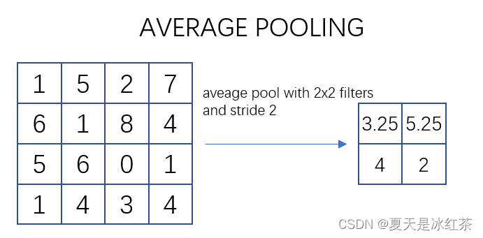
如上图所示，描述的是对一个 4x4 的特征图邻域内的数值进行操作。使用了一个 2x2 的滤波器，步长为2进行扫描，计算邻域内数值的平均值并将其输出到下一层。这种操作被称为平均池化（Mean Pooling）。

"""
Copyright (c) 2023, Auorui.
All rights reserved.

The Torch implementation of average pooling and maximum pooling has been compared with the official Torch implementation
"""
import torch
import torch.nn as nn

__all__ = ["MaxPool2d", "AvgPool2d"]

class MaxPool2d(nn.Module):
    """
    池化层计算公式:
        output_size = [(input_size−kernel_size) // stride + 1]
    """
    def __init__(self, kernel_size, stride):
        super(MaxPool2d, self).__init__()
        self.kernel_size = kernel_size
        self.stride = stride

    def max_pool2d(self, input_tensor, kernel_size, stride):
        batch_size, channels, height, width = input_tensor.size()
        output_height = (height - kernel_size) // stride + 1
        output_width = (width - kernel_size) // stride + 1
        output_tensor = torch.zeros(batch_size, channels, output_height, output_width)

        for i in range(output_height):
            for j in range(output_width):
                # 获取输入张量中与池化窗口对应的部分
                window = input_tensor[:, :,
                         i * stride: i * stride + kernel_size, j * stride: j * stride + kernel_size]
                output_tensor[:, :, i, j] = torch.max(window.reshape(batch_size, channels, -1), dim=2)[0]
        return output_tensor

    def forward(self, input_tensor):
        return self.max_pool2d(input_tensor, kernel_size=self.kernel_size, stride=self.stride)


class AvgPool2d(nn.Module):
    """
    池化层计算公式:
        output_size = [(input_size−kernel_size) // stride + 1]
    """
    def __init__(self, kernel_size, stride):
        super(AvgPool2d, self).__init__()
        self.kernel_size = kernel_size
        self.stride = stride

    def avg_pool2d(self, input_tensor, kernel_size, stride):
        batch_size, channels, height, width = input_tensor.size()
        output_height = (height - kernel_size) // stride + 1
        output_width = (width - kernel_size) // stride + 1
        output_tensor = torch.zeros(batch_size, channels, output_height, output_width)

        for i in range(output_height):
            for j in range(output_width):
                # 获取输入张量中与池化窗口对应的部分
                window = input_tensor[:, :,
                         i * stride: i * stride + kernel_size, j * stride:j * stride + kernel_size]
                output_tensor[:, :, i, j] = torch.mean(window.reshape(batch_size, channels, -1), dim=2)
        return output_tensor

    def forward(self, input_tensor):
        return self.avg_pool2d(input_tensor, kernel_size=self.kernel_size, stride=self.stride)


if __name__=="__main__":
    # input_data = torch.rand((1, 3, 3, 3))
    input_data = torch.Tensor([[[[0.3939, 0.8964, 0.3681],
                               [0.5134, 0.3780, 0.0047],
                               [0.0681, 0.0989, 0.5962]],
                              [[0.7954, 0.4811, 0.3329],
                               [0.8804, 0.3986, 0.3561],
                               [0.2797, 0.3672, 0.6508]],
                              [[0.6309, 0.1340, 0.0564],
                               [0.3101, 0.9927, 0.5554],
                               [0.0947, 0.2305, 0.8299]]]])

    print(input_data.shape)

    kernel_size = 3
    stride = 1
    MaxPool2d1 = nn.MaxPool2d(kernel_size, stride)
    output_data_with_torch_max = MaxPool2d1(input_data)
    AvgPool2d1 = nn.AvgPool2d(kernel_size, stride)
    output_data_with_torch_avg = AvgPool2d1(input_data)
    AvgPool2d2 = AvgPool2d(kernel_size, stride)
    output_data_with_torch_Avg = AvgPool2d2(input_data)
    MaxPool2d2 = MaxPool2d(kernel_size, stride)
    output_data_with_torch_Max = MaxPool2d2(input_data)
    # output_data_with_max = max_pool2d(input_data, kernel_size, stride)
    # output_data_with_avg = avg_pool2d(input_data, kernel_size, stride)

    print("\ntorch.nn pooling Output:")
    print(output_data_with_torch_max,"\n",output_data_with_torch_max.size())
    print(output_data_with_torch_avg,"\n",output_data_with_torch_avg.size())
    print("\npooling Output:")
    print(output_data_with_torch_Max,"\n",output_data_with_torch_Max.size())
    print(output_data_with_torch_Avg,"\n",output_data_with_torch_Avg.size())
    # 直接使用bool方法判断会因为浮点数的原因出现偏差
    print(torch.allclose(output_data_with_torch_max,output_data_with_torch_Max))
    print(torch.allclose(output_data_with_torch_avg,output_data_with_torch_Avg))
    # tensor([[[[0.8964]],       # output_data_with_max
    #          [[0.8804]],
    #          [[0.9927]]]])
    # tensor([[[[0.3686]],       # output_data_with_avg
    #           [[0.5047]],
    #           [[0.4261]]]])

在这里，简单地与PyTorch官方的实现进行了比对，成功的进行复现。

跨步卷积

import torch
import torch.nn as nn

class StridedConvolution(nn.Module):
    def __init__(self, in_channels, out_channels, kernel_size=3, stride=2, is_relu=True):
        super(StridedConvolution, self).__init__()
        self.conv = nn.Conv2d(in_channels, out_channels, kernel_size=kernel_size, stride=stride, padding=1)
        self.relu = nn.ReLU(inplace=True)
        self.is_relu = is_relu

    def forward(self, x):
        x = self.conv(x)
        if self.is_relu:
            x = self.relu(x)
        return x

if __name__ == '__main__':
    input_data = torch.rand((1, 3, 64, 64))
    strided_conv = StridedConvolution(3, 64)
    output_data = strided_conv(input_data)
    print("Input shape:", input_data.shape)
    print("Output shape:", output_data.shape)

对输入进行跨步卷积，并根据 is_relu 参数选择是否添加ReLU激活函数。在构建卷积神经网络时经常被用于下采样步骤，以减小特征图的尺寸。

Haar小波下采样

这一部分就直接参考的作者的代码，与池化不同的是，这里它是要指定输入输出几个通道。

"""
Haar Wavelet-based Downsampling (HWD)

Original address of the paper: https://www.sciencedirect.com/science/article/abs/pii/S0031320323005174
Code reference: https://github.com/apple1986/HWD/tree/main
"""
import torch
import torch.nn as nn
from pytorch_wavelets import DWTForward

class HWDownsampling(nn.Module):
    def __init__(self, in_channel, out_channel):
        super(HWDownsampling, self).__init__()
        self.wt = DWTForward(J=1, wave='haar', mode='zero')
        self.conv_bn_relu = nn.Sequential(
            nn.Conv2d(in_channel * 4, out_channel, kernel_size=1, stride=1),
            nn.BatchNorm2d(out_channel),
            nn.ReLU(inplace=True),
        )

    def forward(self, x):
        yL, yH = self.wt(x)
        y_HL = yH[0][:, :, 0, ::]
        y_LH = yH[0][:, :, 1, ::]
        y_HH = yH[0][:, :, 2, ::]
        x = torch.cat([yL, y_HL, y_LH, y_HH], dim=1)
        x = self.conv_bn_relu(x)
        return x


if __name__ == '__main__':
    downsampling_layer = HWDownsampling(3, 64)
    input_data = torch.rand((1, 3, 64, 64))
    output_data = downsampling_layer(input_data)
    print("Input shape:", input_data.shape)
    print("Output shape:", output_data.shape)

Haar小波变换是一种基于小波的信号处理方法，它将信号分解成低频和细节高频两个部分。在图像处理中，Haar小波通常用于图像压缩和特征提取，代码中使用的DWTForward模块中离散小波变换，通过选择 yH 中的不同方向上的高频分量，构建了新的特征图。将原始低频分量 yL 与新构建的高频分量拼接在一起。最后通过一个包含卷积、批归一化和ReLU激活函数的序列处理最终的特征图。

实验验证

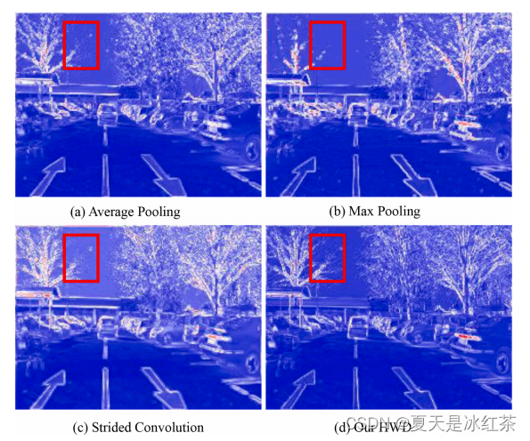
这是作者论文中做的实验，这样看起来，似乎HWD在细节上确实是比池化和跨步卷积效果要好。

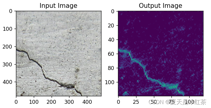
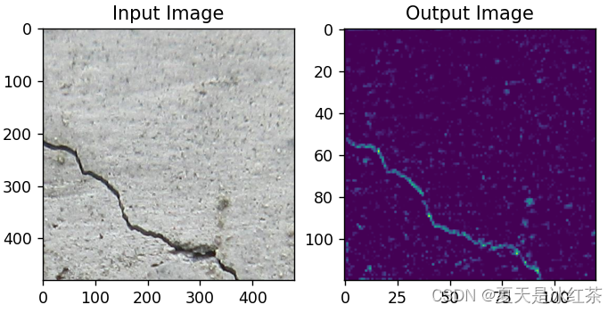
这里因为我也用我自己的数据进行了实验：

最大池化效果

平均池化效果

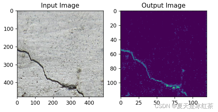
跨步卷积效果

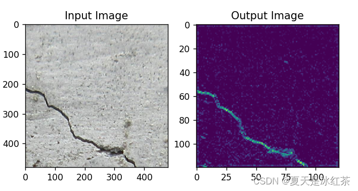
HDW效果

从肉眼上来看，HDW的效果确实要比其他的效果要好一些。

下面是我做实验的代码，感兴趣的可以在自己的数据上面进行实验，我觉得用于交通和医学上应该会有比较好的效果。

import cv2
import torch
import torchvision.transforms as transforms
import matplotlib.pyplot as plt
import torch.nn as nn
from pytorch_wavelets import DWTForward

class StridedConvolution(nn.Module):
    def __init__(self, in_channels, out_channels, kernel_size=3, stride=2, is_relu=True):
        super(StridedConvolution, self).__init__()
        self.conv = nn.Conv2d(in_channels, out_channels, kernel_size=kernel_size, stride=stride, padding=1)
        self.relu = nn.ReLU(inplace=True)
        self.is_relu = is_relu

    def forward(self, x):
        x = self.conv(x)
        if self.is_relu:
            x = self.relu(x)
        return x

class HWDownsampling(nn.Module):
    def __init__(self, in_channel, out_channel):
        super(HWDownsampling, self).__init__()
        self.wt = DWTForward(J=1, wave='haar', mode='zero')
        self.conv_bn_relu = nn.Sequential(
            nn.Conv2d(in_channel * 4, out_channel, kernel_size=1, stride=1),
            nn.BatchNorm2d(out_channel),
            nn.ReLU(inplace=True),
        )

    def forward(self, x):
        yL, yH = self.wt(x)
        y_HL = yH[0][:, :, 0, ::]
        y_LH = yH[0][:, :, 1, ::]
        y_HH = yH[0][:, :, 2, ::]
        x = torch.cat([yL, y_HL, y_LH, y_HH], dim=1)
        x = self.conv_bn_relu(x)
        return x

class DeeperCNN(nn.Module):
    def __init__(self):
        super(DeeperCNN, self).__init__()
        self.conv1 = nn.Conv2d(3, 16, kernel_size=3, stride=1, padding=1)
        self.batch_norm1 = nn.BatchNorm2d(16)
        self.relu = nn.ReLU()
        self.pool1 = nn.MaxPool2d(kernel_size=2, stride=2)
        # self.pool1 = nn.AvgPool2d(kernel_size=2, stride=2)
        # self.pool1 = HWDownsampling(16, 16)
        self.pool1 = StridedConvolution(16, 16, is_relu=True)

        self.conv2 = nn.Conv2d(16, 32, kernel_size=3, stride=1, padding=1)
        self.batch_norm2 = nn.BatchNorm2d(32)
        # self.pool2 = nn.MaxPool2d(kernel_size=2, stride=2)
        # self.pool2 = nn.AvgPool2d(kernel_size=2, stride=2)
        # self.pool2 = HWDownsampling(32, 32)
        self.pool2 = StridedConvolution(32, 32, is_relu=True)

        self.conv6 = nn.Conv2d(32, 1, kernel_size=3, stride=1, padding=1)

    def forward(self, x):
        x = self.pool1(self.relu(self.batch_norm1(self.conv1(x))))
        print(x.shape)
        x = self.pool2(self.relu(self.batch_norm2(self.conv2(x))))
        print(x.shape)
        x = self.conv6(x)
        return x

image_path = r'D:\PythonProject\Crack_classification_training_script\data\base\val\crack\2416.png'
image = cv2.imread(image_path)
image = cv2.cvtColor(image, cv2.COLOR_BGR2RGB)

transform = transforms.Compose([transforms.ToTensor()])
input_image = transform(image).unsqueeze(0)
import numpy as np
model = DeeperCNN()
output = model(input_image)
print("Output shape:", output.shape)

input_image = input_image.squeeze(0).permute(1, 2, 0).numpy()
output_image = output.squeeze(0).permute(1, 2, 0).detach().numpy()
output_image = output_image / output_image.max()
output_image = np.clip(output_image, 0, 1)

plt.subplot(1, 2, 1)
plt.imshow(input_image)
plt.title('Input Image')

plt.subplot(1, 2, 2)
plt.imshow(output_image)
plt.title('Output Image')

plt.show()