OpenCV PCA介绍

泠山

已于 2023-10-25 10:08:16 修改

阅读量1.7k

点赞数 2

分类专栏：计算机视觉文章标签： opencv 计算机视觉 python

于 2022-08-23 11:05:21 首次发布

本文链接：https://blog.csdn.net/qq_28087491/article/details/126478846

版权

计算机视觉专栏收录该内容

19 篇文章 9 订阅

订阅专栏

OpenCV PCA介绍

1. 什么是PCA
2. 特征向量与特征值如何计算
3. 源代码
- 3.1 代码解释
- 3.2 结果

相关文章：

异值分解SVD、主成分分析PCA、行列式

这篇文章将介绍如何去使用 OpenCV 类：cv::PCA 来计算目标方向。

1. 什么是PCA

主成分分析(PCA)是一个统计过程，提取一个数据集最重要的特征。
在这里插入图片描述
假设有一组2D点，如上图所示。每个维度对应一个感兴趣的特征。有些人可能会说，这些点的设置顺序是随机的。然而，如果仔细观察，会发现这里有一个很难忽略的线性模式(由蓝色线表示)。主成分分析的一个关键点是降维。降维是减少给定数据集的维数的过程。例如，在上述情况下，可以将一组点近似为一条直线，从而将给定点的维数从2D降至1D。

此外还可以看到，这些点沿着蓝线变化最大，比沿着特征1或特征2轴变化更大。这意味着，如果你知道一个点沿着蓝色直线的位置，你就比只知道它在特征1轴或特征2轴上的位置有更多的信息。

因此，PCA允许我们找到数据变化最大的方向。事实上，在图中点的集合上运行主成分分析的结果由两个称为特征向量(eigenvector)的向量组成，它们是数据集的主成分。
在这里插入图片描述每个特征向量的大小被编码到对应的特征值中，表明数据沿着主成分变化的程度。特征向量的起点是数据集中所有点的中心。将PCA应用于N维数据集，得到N个N维特征向量、N个特征值和1个N维中心点。

2. 特征向量与特征值如何计算

我们的目标是将一个给定的 $p$ 维数据集 $\mathbf{X}$ 转换为另一个更小维度 $L$ 的数据集 Y。同样地，我们寻找矩阵 Y，其中 Y 是矩阵 $\mathbf{X}$ 的Karhunen-Loève变换(KLT)：
$\mathbf{Y}=\mathbb{K} \mathbb{L T}\{\mathbf{X}\}$

2.1 组织数据集

假设你的数据包含 $p$ 个变量的一组观察数据，你想要减少数据，以便每个观察数据可以只用 $L$ 个变量来描述， $L < p$ 。进一步假设，数据被排列为 $n$ 个数据向量 $x_1…x_n$ ，其中每一个 $x_i$ 代表 $p$ 个变量的一个组合观测量。

将 $x_1…x_n$ 写入行向量，每一个都有 $p$ 列；
将行向量放入一个单独的维度为 $n\times p$ 的矩阵 $\mathbf{X}$ 。

2.2 计算经验均值

找出每个维度 $j = 1, ..., p$ 的经验平均值；
将计算的平均值放入维度为 $p \times 1$ 的经验均值向量 $\mathbf{u}$ 中。
$\mathbf{u}[\mathbf{j}]=\frac{1}{n} \sum_{i=1}^{n} \mathbf{X}[\mathbf{i}, \mathbf{j}]$

2.3 计算与均值的偏差

平均值减法是解决方案的一个组成部分，以找到一个主成分基(principal component basis)，以最小化均方误差的逼近数据。因此，我们使用如下方法找到数据中心：

从数据矩阵 $\mathbf{X}$ 的每一行中减去经验均值向量 $\mathbf{u}$ 。
储存减去平均值的数据进 $n\times p$ 的矩阵 $\mathbf{B}$ 。
$\mathbf{B}=\mathbf{X}-\mathbf{h u}^{\mathbf{T}}$

其中 $\mathbf{h}$ 是一个值全为 $1$ 的 $n\times 1$ 的列向量：
$\ldots, n$

2.4 寻找协方差矩阵

由矩阵 $\mathbf{B}$ 与自身的外积求 $p \times p$ 经验协方差矩阵(empirical covariance matrix) $\mathbf{C}$ ：
$\mathbf{C}=\frac{1}{n-1} \mathbf{B}^{*} \cdot \mathbf{B}$

其中*为共轭转置算子(conjugate transpose operator)。注意，如果 $\mathbf{B}$ 完全由实数组成，这是许多应用中的情况，“共轭转置”与通常的转置相同。

2.5 求协方差矩阵的特征向量和特征值

计算将协方差矩阵 $\mathbf{C}$ 对角化的特征向量矩阵 $\mathbf{V}$ ：
$\mathbf{V}^{-1} \mathbf{C V}=\mathbf{D}$

其中 $\mathbf{D}$ 是 $\mathbf{C}$ 的特征值的对角矩阵(diagonal matrix)。
矩阵 $\mathbf{D}$ 将采用 $p \times p$ 对角矩阵的形式：
$l]=\left\{\begin{array}{c} \lambda_{k}, k=l \\ 0, k \neq l \end{array}\right.$

这里， $λ_j$ 是协方差矩阵 $\mathbf{C}$ 的第 $j$ 个特征值。
矩阵 $\mathbf{V}$ 的维数也是 $p\times p$ ，包含 $p$ 个列向量，每个列向量的长度为 $p$ ，它们表示协方差矩阵 $\mathbf{C}$ 的 $p$ 个特征向量。
特征值和特征向量是有序且配对的。第 $j$ 个特征值对应于第 $j$ 个特征向量。

3. 源代码

#include "opencv2/core.hpp"
#include "opencv2/imgproc.hpp"
#include "opencv2/highgui.hpp"
#include <iostream>
using namespace std;
using namespace cv;
// Function declarations
void drawAxis(Mat&, Point, Point, Scalar, const float);
double getOrientation(const vector<Point> &, Mat&);
void drawAxis(Mat& img, Point p, Point q, Scalar colour, const float scale = 0.2)
{
    double angle = atan2( (double) p.y - q.y, (double) p.x - q.x ); // angle in radians
    double hypotenuse = sqrt( (double) (p.y - q.y) * (p.y - q.y) + (p.x - q.x) * (p.x - q.x));
    // Here we lengthen the arrow by a factor of scale
    q.x = (int) (p.x - scale * hypotenuse * cos(angle));
    q.y = (int) (p.y - scale * hypotenuse * sin(angle));
    line(img, p, q, colour, 1, LINE_AA);
    // create the arrow hooks
    p.x = (int) (q.x + 9 * cos(angle + CV_PI / 4));
    p.y = (int) (q.y + 9 * sin(angle + CV_PI / 4));
    line(img, p, q, colour, 1, LINE_AA);
    p.x = (int) (q.x + 9 * cos(angle - CV_PI / 4));
    p.y = (int) (q.y + 9 * sin(angle - CV_PI / 4));
    line(img, p, q, colour, 1, LINE_AA);
}
double getOrientation(const vector<Point> &pts, Mat &img)
{
    //Construct a buffer used by the pca analysis
    int sz = static_cast<int>(pts.size());
    Mat data_pts = Mat(sz, 2, CV_64F);
    for (int i = 0; i < data_pts.rows; i++)
    {
        data_pts.at<double>(i, 0) = pts[i].x;
        data_pts.at<double>(i, 1) = pts[i].y;
    }
    //Perform PCA analysis
    PCA pca_analysis(data_pts, Mat(), PCA::DATA_AS_ROW);
    //Store the center of the object
    Point cntr = Point(static_cast<int>(pca_analysis.mean.at<double>(0, 0)),
                      static_cast<int>(pca_analysis.mean.at<double>(0, 1)));
    //Store the eigenvalues and eigenvectors
    vector<Point2d> eigen_vecs(2);
    vector<double> eigen_val(2);
    for (int i = 0; i < 2; i++)
    {
        eigen_vecs[i] = Point2d(pca_analysis.eigenvectors.at<double>(i, 0),
                                pca_analysis.eigenvectors.at<double>(i, 1));
        eigen_val[i] = pca_analysis.eigenvalues.at<double>(i);
    }
    // Draw the principal components
    circle(img, cntr, 3, Scalar(255, 0, 255), 2);
    Point p1 = cntr + 0.02 * Point(static_cast<int>(eigen_vecs[0].x * eigen_val[0]), static_cast<int>(eigen_vecs[0].y * eigen_val[0]));
    Point p2 = cntr - 0.02 * Point(static_cast<int>(eigen_vecs[1].x * eigen_val[1]), static_cast<int>(eigen_vecs[1].y * eigen_val[1]));
    drawAxis(img, cntr, p1, Scalar(0, 255, 0), 1);
    drawAxis(img, cntr, p2, Scalar(255, 255, 0), 5);
    double angle = atan2(eigen_vecs[0].y, eigen_vecs[0].x); // orientation in radians
    return angle;
}
int main(int argc, char** argv)
{
    // Load image
    CommandLineParser parser(argc, argv, "{@input | pca_test1.jpg | input image}");
    parser.about( "This program demonstrates how to use OpenCV PCA to extract the orientation of an object.\n" );
    parser.printMessage();
    Mat src = imread( samples::findFile( parser.get<String>("@input") ) );
    // Check if image is loaded successfully
    if(src.empty())
    {
        cout << "Problem loading image!!!" << endl;
        return EXIT_FAILURE;
    }
    imshow("src", src);
    // Convert image to grayscale
    Mat gray;
    cvtColor(src, gray, COLOR_BGR2GRAY);
    // Convert image to binary
    Mat bw;
    threshold(gray, bw, 50, 255, THRESH_BINARY | THRESH_OTSU);
    // Find all the contours in the thresholded image
    vector<vector<Point> > contours;
    findContours(bw, contours, RETR_LIST, CHAIN_APPROX_NONE);
    for (size_t i = 0; i < contours.size(); i++)
    {
        // Calculate the area of each contour
        double area = contourArea(contours[i]);
        // Ignore contours that are too small or too large
        if (area < 1e2 || 1e5 < area) continue;
        // Draw each contour only for visualisation purposes
        drawContours(src, contours, static_cast<int>(i), Scalar(0, 0, 255), 2);
        // Find the orientation of each shape
        getOrientation(contours[i], src);
    }
    imshow("output", src);
    waitKey();
    return EXIT_SUCCESS;
}

3.1 代码解释

读取图像并将其转换为二进制
在这里，我们应用必要的预处理程序，以便能够检测感兴趣的对象。

 // Load image
 CommandLineParser parser(argc, argv, "{@input | pca_test1.jpg | input image}");
 parser.about( "This program demonstrates how to use OpenCV PCA to extract the orientation of an object.\n" );
 parser.printMessage();
 Mat src = imread( samples::findFile( parser.get<String>("@input") ) );
 // Check if image is loaded successfully
 if(src.empty())
 {
     cout << "Problem loading image!!!" << endl;
     return EXIT_FAILURE;
 }
 imshow("src", src);
 // Convert image to grayscale
 Mat gray;
 cvtColor(src, gray, COLOR_BGR2GRAY);
 // Convert image to binary
 Mat bw;
 threshold(gray, bw, 50, 255, THRESH_BINARY | THRESH_OTSU);

提取感兴趣的对象
然后根据轮廓大小找到并过滤轮廓，得到剩余轮廓的方向。

// Find all the contours in the thresholded image
vector<vector<Point> > contours;
findContours(bw, contours, RETR_LIST, CHAIN_APPROX_NONE);
for (size_t i = 0; i < contours.size(); i++)
{
    // Calculate the area of each contour
    double area = contourArea(contours[i]);
    // Ignore contours that are too small or too large
    if (area < 1e2 || 1e5 < area) continue;
    // Draw each contour only for visualisation purposes
    drawContours(src, contours, static_cast<int>(i), Scalar(0, 0, 255), 2);
    // Find the orientation of each shape
    getOrientation(contours[i], src);
}

提取方向
方向是通过调用 getOrientation() 函数来提取的，该函数执行所有的PCA过程。

//Construct a buffer used by the pca analysis
int sz = static_cast<int>(pts.size());
Mat data_pts = Mat(sz, 2, CV_64F);
for (int i = 0; i < data_pts.rows; i++)
{
    data_pts.at<double>(i, 0) = pts[i].x;
    data_pts.at<double>(i, 1) = pts[i].y;
}
//Perform PCA analysis
PCA pca_analysis(data_pts, Mat(), PCA::DATA_AS_ROW);
//Store the center of the object
Point cntr = Point(static_cast<int>(pca_analysis.mean.at<double>(0, 0)),
                  static_cast<int>(pca_analysis.mean.at<double>(0, 1)));
//Store the eigenvalues and eigenvectors
vector<Point2d> eigen_vecs(2);
vector<double> eigen_val(2);
for (int i = 0; i < 2; i++)
{
    eigen_vecs[i] = Point2d(pca_analysis.eigenvectors.at<double>(i, 0),
                            pca_analysis.eigenvectors.at<double>(i, 1));
    eigen_val[i] = pca_analysis.eigenvalues.at<double>(i);
}

首先，数据需要排列在一个大小为 $n \times 2$ 的矩阵中，其中 $n$ 是我们所拥有的数据点的数量。然后我们就可以进行主成分分析。计算出的均值(即质心)存储在cntr变量中，特征向量和特征值存储在相应的 std::vector 中。

可视化结果
最终的结果通过 drawaaxis() 函数可视化，其中的主成分用直线绘制，每个特征向量乘以其特征值并平移到平均位置。

// Draw the principal components
circle(img, cntr, 3, Scalar(255, 0, 255), 2);
Point p1 = cntr + 0.02 * Point(static_cast<int>(eigen_vecs[0].x * eigen_val[0]), static_cast<int>(eigen_vecs[0].y * eigen_val[0]));
Point p2 = cntr - 0.02 * Point(static_cast<int>(eigen_vecs[1].x * eigen_val[1]), static_cast<int>(eigen_vecs[1].y * eigen_val[1]));
drawAxis(img, cntr, p1, Scalar(0, 255, 0), 1);
drawAxis(img, cntr, p2, Scalar(255, 255, 0), 5);
double angle = atan2(eigen_vecs[0].y, eigen_vecs[0].x); // orientation in radians

double angle = atan2( (double) p.y - q.y, (double) p.x - q.x ); // angle in radians
double hypotenuse = sqrt( (double) (p.y - q.y) * (p.y - q.y) + (p.x - q.x) * (p.x - q.x));
// Here we lengthen the arrow by a factor of scale
q.x = (int) (p.x - scale * hypotenuse * cos(angle));
q.y = (int) (p.y - scale * hypotenuse * sin(angle));
line(img, p, q, colour, 1, LINE_AA);
// create the arrow hooks
p.x = (int) (q.x + 9 * cos(angle + CV_PI / 4));
p.y = (int) (q.y + 9 * sin(angle + CV_PI / 4));
line(img, p, q, colour, 1, LINE_AA);
p.x = (int) (q.x + 9 * cos(angle - CV_PI / 4));
p.y = (int) (q.y + 9 * sin(angle - CV_PI / 4));
line(img, p, q, colour, 1, LINE_AA);

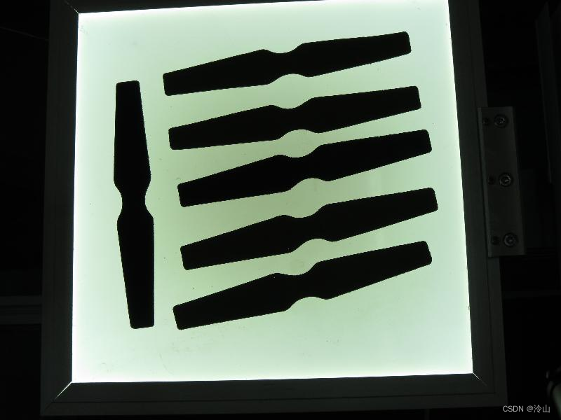
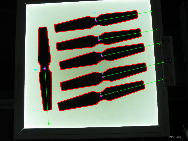
3.2 结果

该代码打开一个图像，找到检测到的感兴趣的对象的方向，然后通过绘制检测到的感兴趣的对象的轮廓、中心点和关于提取的方向的x轴、y轴来可视化结果。

泠山

关注

2
点赞
踩
11

收藏

觉得还不错? 一键收藏
打赏
0
评论
OpenCV PCA介绍

主成分分析(PCA)是一个统计过程，提取一个数据集最重要的特征。假设有一组2D点，如上图所示。每个维度对应一个感兴趣的特征。有些人可能会说，这些点的设置顺序是随机的。然而，如果仔细观察，会发现这里有一个很难忽略的线性模式(由蓝色线表示)。主成分分析的一个关键点是降维。降维是减少给定数据集的维数的过程。例如，在上述情况下，可以将一组点近似为一条直线，从而将给定点的维数从2D降至1D。此外还可以看到，这些点沿着蓝线变化最大，比沿着特征1或特征2轴变化更大。
复制链接

扫一扫