轨迹分析分化 速率分析 monocle slingshot安装 seurat pseudotime

Pseudotime analysis with slingshothttps://bustools.github.io/BUS_notebooks_R/slingshot.html

GitHub - satijalab/seurat-wrappers: Community-provided extensions to Seurat 

Slingshot: Trajectory Inference for Single-Cell Data

Installationhttps://bioconductor.org/packages/release/bioc/html/slingshot.html

To install this package, start R (version "4.3") and enter:

if (!require("BiocManager", quietly = TRUE))
    install.packages("BiocManager")

BiocManager::install("slingshot")

Pseudotime analysis with slingshot

Lambda Moses

2020-01-21

 workflowr 

• Summary
• Checks 
• Past versions

Last updated: 2020-01-21

Checks:  7  0

Knit directory: BUS_notebooks_R/ 

This reproducible R Markdown analysis was created with workflowr (version 1.6.0). The Checks tab describes the reproducibility checks that were applied when the results were created. The Past versions tab lists the development history.

---

Introduction

This notebook does pseudotime analysis of the 10x 10k neurons from an E18 mouse using slingshot, which is on Bioconductor. The notebook begins with pre-processing of the reads with the kallisto | bustools workflow Like Monocle 2 DDRTree, slingshot builds a minimum spanning tree, but while Monocle 2 builds the tree from individual cells, slingshot does so with clusters. slingshot is also the top rated trajectory inference method in the dynverse paper.

In the kallisto | bustools paper, I used the docker container for slingshot provided by dynverse for pseudotime analysis, because dynverse provides unified interface to dozens of different trajectory inference (TI) methods via docker containers, making it easy to try other methods without worrying about installing dependencies. Furthermore, dynverse provides metrics to evaluate TI methods. However, the docker images provided by dynverse do not provide users with the full range of options available from the TI methods themselves. For instance, while any dimension reduction and any kind of clustering can be used for slingshot, dynverse chose PCA and partition around medoids (PAM) clustering for us (see the source code here). So in this notebook, we will directly use slingshot rather than via dynverse.

The gene count matrix of the 10k neuron dataset has already been generated with the kallisto | bustools pipeline and filtered for the Monocle 2 notebook. Cell types have also been annotated with SingleR in that notebook. Please refer to the first 3 main sections of that notebook for instructions on how to use kallisto | bustools, remove empty droplets, and annotate cell types.

Packages slingshot and BUSpaRse are on Bioconductor (3.10). The other packages are on CRAN.

library(slingshot)
library(BUSpaRse)
library(tidyverse)
library(tidymodels)
library(Seurat)
library(scales)
library(viridis)
library(Matrix)

Loading the matrix

The filtered gene count matrix and the cell annotation were saved from the Monocle 2 notebook.

annot <- readRDS("./output/neuron10k/cell_type.rds")
mat_filtered <- readRDS("./output/neuron10k/mat_filtered.rds")

Just to show the structures of those 2 objects:

dim(mat_filtered)

#> [1] 23516 11037

class(mat_filtered)

#> [1] "dgCMatrix"
#> attr(,"package")
#> [1] "Matrix"

Row names are Ensembl gene IDs.

head(rownames(mat_filtered))

#> [1] "ENSMUSG00000094619.2"  "ENSMUSG00000095646.1"  "ENSMUSG00000092401.3" 
#> [4] "ENSMUSG00000109389.1"  "ENSMUSG00000092212.3"  "ENSMUSG00000079293.11"

head(colnames(mat_filtered))

#> [1] "AAACCCACACGCGGTT" "AAACCCACAGCATACT" "AAACCCACATACCATG" "AAACCCAGTCGCACAC"
#> [5] "AAACCCAGTGCACATT" "AAACCCAGTGGTAATA"

str(annot)

#> List of 10
#>  $ scores       : num [1:11037, 1:28] 0.188 0.194 0.182 0.267 0.187 ...
#>   ..- attr(*, "dimnames")=List of 2
#>   .. ..$ : chr [1:11037] "AAACCCACACGCGGTT" "AAACCCACAGCATACT" "AAACCCACATACCATG" "AAACCCAGTCGCACAC" ...
#>   .. ..$ : chr [1:28] "Adipocytes" "aNSCs" "Astrocytes" "Astrocytes activated" ...
#>  $ labels       : chr [1:11037, 1] "NPCs" "NPCs" "NPCs" "NPCs" ...
#>   ..- attr(*, "dimnames")=List of 2
#>   .. ..$ : chr [1, 1:11037] "AAACCCACACGCGGTT" "AAACCCACAGCATACT" "AAACCCACATACCATG" "AAACCCAGTCGCACAC" ...
#>   .. ..$ : NULL
#>  $ r            : num [1:11037, 1:358] 0.187 0.197 0.179 0.251 0.171 ...
#>   ..- attr(*, "dimnames")=List of 2
#>   .. ..$ : chr [1:11037] "AAACCCACACGCGGTT" "AAACCCACAGCATACT" "AAACCCACATACCATG" "AAACCCAGTCGCACAC" ...
#>   .. ..$ : chr [1:358] "ERR525589Aligned" "ERR525592Aligned" "SRR275532Aligned" "SRR275534Aligned" ...
#>  $ pval         : Named num [1:11037] 0.0428 0.058 0.0383 0.0111 0.0327 ...
#>   ..- attr(*, "names")= chr [1:11037] "AAACCCACACGCGGTT" "AAACCCACAGCATACT" "AAACCCACATACCATG" "AAACCCAGTCGCACAC" ...
#>  $ labels1      : chr [1:11037, 1] "NPCs" "NPCs" "NPCs" "NPCs" ...
#>   ..- attr(*, "dimnames")=List of 2
#>   .. ..$ : chr [1:11037] "AAACCCACACGCGGTT" "AAACCCACAGCATACT" "AAACCCACATACCATG" "AAACCCAGTCGCACAC" ...
#>   .. ..$ : NULL
#>  $ labels1.thres: chr [1:11037] "NPCs" "X" "NPCs" "NPCs" ...
#>  $ cell.names   : chr [1:11037] "AAACCCACACGCGGTT" "AAACCCACAGCATACT" "AAACCCACATACCATG" "AAACCCAGTCGCACAC" ...
#>  $ quantile.use : num 0.8
#>  $ types        : chr [1:358] "Adipocytes" "Adipocytes" "Adipocytes" "Adipocytes" ...
#>  $ method       : chr "single"

To prevent endothelial cells, erythrocytes, immune cells, and fibroblasts from being mistaken as very differentiated cell types derived from neural stem cells, we will only keep cells with a label for the neural or glial lineage. This can be a problem as slingshot does not support multiple disconnected trajectories.

ind <- annot$labels %in% c("NPCs", "Neurons", "OPCs", "Oligodendrocytes", 
                           "qNSCs", "aNSCs", "Astrocytes", "Ependymal")
cells_use <- annot$cell.names[ind]
mat_filtered <- mat_filtered[, cells_use]

Meaning of the acronyms:

• NPCs: Neural progenitor cells
• OPCs: Oligodendrocyte progenitor cells
• qNSCs: Quiescent neural stem cells
• aNSCs: Active neural stem cells

Since we will do differential expression and gene symbols are more human readable than Ensembl gene IDs, we will get the corresponding gene symbols from Ensembl.

gns <- tr2g_ensembl(species = "Mus musculus", use_gene_name = TRUE, 
                    ensembl_version = 97)[,c("gene", "gene_name")] %>% 
  distinct()

#> Querying biomart for transcript and gene IDs of Mus musculus

#> Cache found

Preprocessing

 

QC

seu <- CreateSeuratObject(mat_filtered) %>% 
  SCTransform() # normalize and scale
# Add cell type annotation to metadata
seu <- AddMetaData(seu, setNames(annot$labels[ind], cells_use), 
                   col.name = "cell_type")

VlnPlot(seu, c("nCount_RNA", "nFeature_RNA"), pt.size = 0.1, ncol = 1, group.by = "cell_type")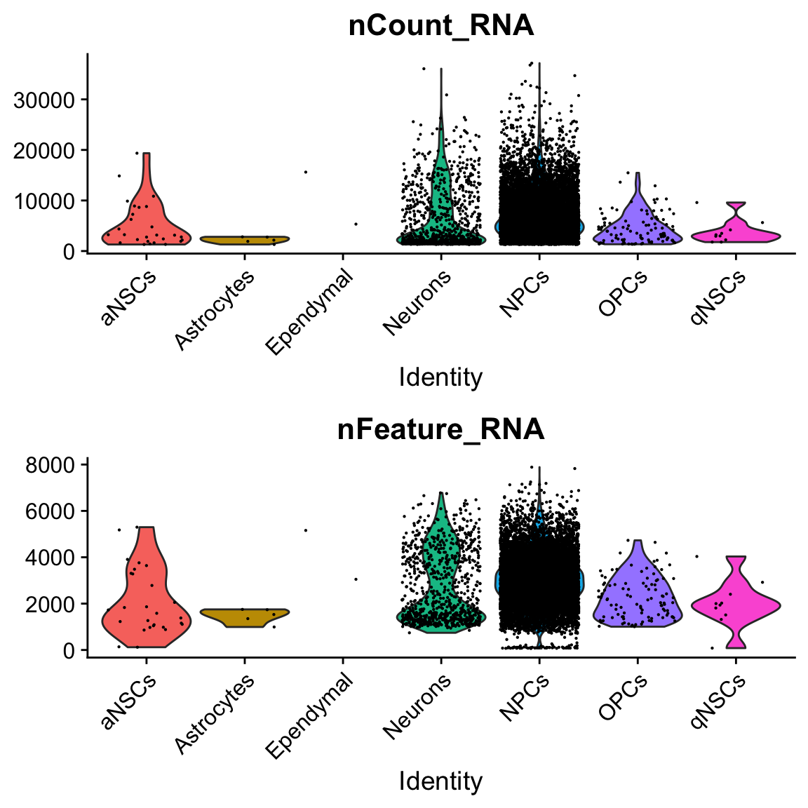

Past versions of vln-1.png

There are only 2 cells labeled ependymal.

ggplot(seu@meta.data, aes(nCount_RNA, nFeature_RNA, color = cell_type)) +
  geom_point(size = 0.5) +
  scale_color_brewer(type = "qual", palette = "Set2", name = "cell type") +
  scale_x_log10() +
  scale_y_log10() +
  theme_bw() +
  # Make points larger in legend
  guides(color = guide_legend(override.aes = list(size = 3))) +
  labs(x = "Total UMI counts", y = "Number of genes detected")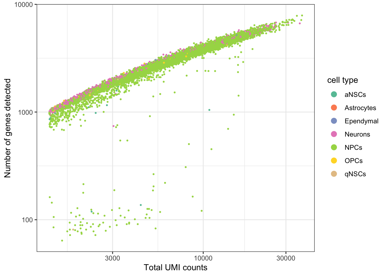

Past versions of qc-1.png

Dimension reduction

seu <- RunPCA(seu, npcs = 70, verbose = FALSE)
ElbowPlot(seu, ndims = 70)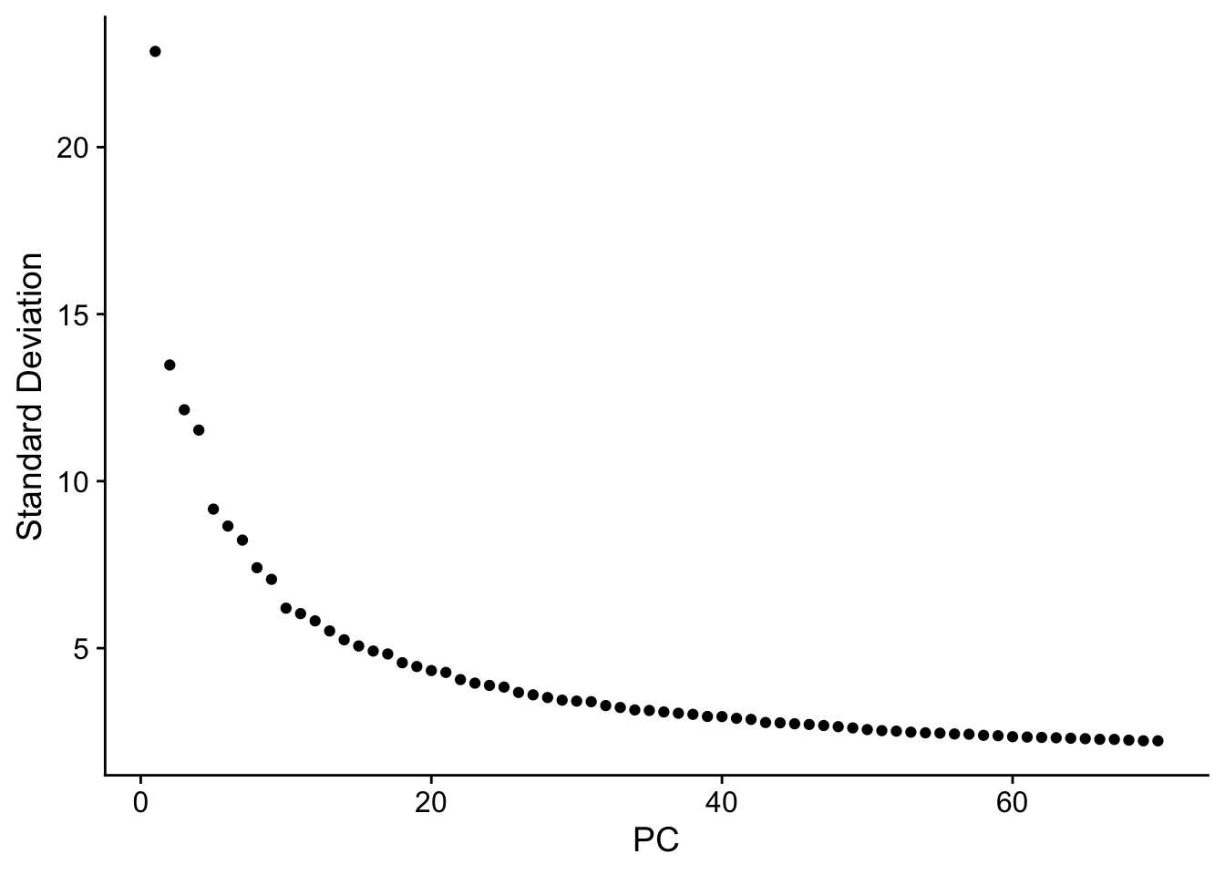

Past versions of elbow-1.png

The y axis is standard deviation (not variance), or the singular values from singular value decomposition on the data performed for PCA.

# Need to use DimPlot due to weird workflowr problem with PCAPlot that calls seu[[wflow.build]]
# and eats up memory. I suspect this is due to the sys.call() in 
# Seurat:::SpecificDimPlot. 
DimPlot(seu, reduction = "pca",
        group.by = "cell_type", pt.size = 0.5, label = TRUE, repel = TRUE) +
  scale_color_brewer(type = "qual", palette = "Set2")

#> Warning: Using `as.character()` on a quosure is deprecated as of rlang 0.3.0.
#> Please use `as_label()` or `as_name()` instead.
#> This warning is displayed once per session.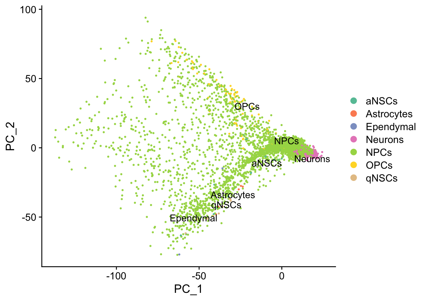

Past versions of pca-1.png

seu <- RunTSNE(seu, dims = 1:50, verbose = FALSE)
DimPlot(seu, reduction = "tsne",
        group.by = "cell_type", pt.size = 0.5, label = TRUE, repel = TRUE) +
  scale_color_brewer(type = "qual", palette = "Set2")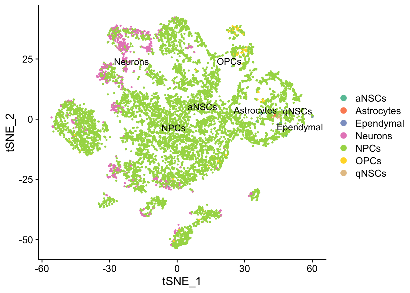

Past versions of tsne-1.png

UMAP can better preserve pairwise distance of cells than tSNE and can better separate cell populations than the first 2 PCs of PCA (Becht et al. 2018), so the TI will be done on UMAP rather than tSNE or PCA. The current CRAN version of Seurat uses the R package uwot rather than the Python version for UMAP.

seu <- RunUMAP(seu, dims = 1:50, seed.use = 4867)

#> Warning: The default method for RunUMAP has changed from calling Python UMAP via reticulate to the R-native UWOT using the cosine metric
#> To use Python UMAP via reticulate, set umap.method to 'umap-learn' and metric to 'correlation'
#> This message will be shown once per session

 

DimPlot(seu, reduction = "umap",
        group.by = "cell_type", pt.size = 0.5, label = TRUE, repel = TRUE) +
  scale_color_brewer(type = "qual", palette = "Set2")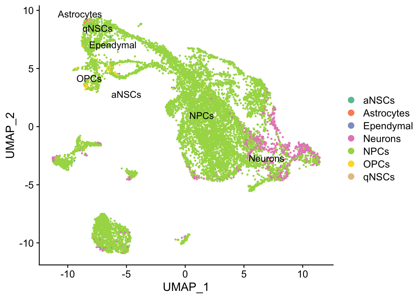

Past versions of umap-1.png

Cell type annotation with SingleR requires a reference with bulk RNA seq data for isolated known cell types. The reference used for cell type annotation here does not differentiate between different types of neural progenitor cells; clustering can further partition the neural progenitor cells. Furthermore, slingshot is based on cluster-wise minimum spanning tree, so finding a good clustering is important to good trajectory inference with slingshot. The clustering algorithm used here is Leiden, which is an improvement over the commonly used Louvain; Leiden communities are guaranteed to be well-connected, while Louvain can lead to poorly connected communities.

names(seu@meta.data)

#> [1] "orig.ident"   "nCount_RNA"   "nFeature_RNA" "nCount_SCT"   "nFeature_SCT"
#> [6] "cell_type"

seu <- FindNeighbors(seu, verbose = FALSE, dims = 1:50)
seu <- FindClusters(seu, algorithm = 4, random.seed = 256, resolution = 1)

#> 10653 singletons identified. 17 final clusters.

DimPlot(seu, pt.size = 0.5, reduction = "umap", group.by = "seurat_clusters", label = TRUE)

Past versions of umap_clust-1.png

Slingshot

Slingshot

Trajectory inference

While the slingshot vignette uses SingleCellExperiment, slingshot can also take a matrix of cell embeddings in reduced dimension as input. We can optionally specify the cluster to start or end the trajectory based on biological knowledge. Here, since quiescent neural stem cells are in cluster 4, the starting cluster would be 4 near the top left of the previous plot.

Here, UMAP projections are used for trajectory inference, as in Monocle 3, for the purpose of visualization. However, I no longer consider this a good idea, due to distortions introduced by UMAP. See this paper for the extent non-linear dimension reduction methods distort the data. The latent dimension of the data is most likely far more than 2 or 3 dimensions, so forcing it down to 2 or 3 dimensions are bound to introduce distortions, just like how projecting the spherical surface of the Earth to 2 dimensions in maps introduces distortions. Furthermore, after the projection, some trajectories are no longer topologically feasible. For instance, imagine a stream coming out of the hole of a doughnut in 3D. This is not possible in 2D, so when that structure is projected to 2D, part of the stream may become buried in the middle of the doughnut, or the doughnut may be broken to allow the stream through, or part of the steam will be intermixed with part of the doughnut though they shouldn’t. I recommend using a larger number of principal components instead, but in that case, the lineages and principal curves can’t be visualized (we can plot the curves within a 2 dimensional subspace, such as the first 2 PCs, but that usually looks like abstract art and isn’t informative about the lineages).

 

sds <- slingshot(Embeddings(seu, "umap"), clusterLabels = seu$seurat_clusters, 
                 start.clus = 4, stretch = 0)

Unfortunately, slingshot does not natively support ggplot2. So this is a function that assigns colors to each cell in base R graphics.

#' Assign a color to each cell based on some value
#' 
#' @param cell_vars Vector indicating the value of a variable associated with cells.
#' @param pal_fun Palette function that returns a vector of hex colors, whose
#' argument is the length of such a vector.
#' @param ... Extra arguments for pal_fun.
#' @return A vector of hex colors with one entry for each cell.
cell_pal <- function(cell_vars, pal_fun,...) {
  if (is.numeric(cell_vars)) {
    pal <- pal_fun(100, ...)
    return(pal[cut(cell_vars, breaks = 100)])
  } else {
    categories <- sort(unique(cell_vars))
    pal <- setNames(pal_fun(length(categories), ...), categories)
    return(pal[cell_vars])
  }
}

We need color palettes for both cell types and Leiden clusters. These would be the same colors seen in the Seurat plots.

cell_colors <- cell_pal(seu$cell_type, brewer_pal("qual", "Set2"))
cell_colors_clust <- cell_pal(seu$seurat_clusters, hue_pal())

What does the inferred trajectory look like compared to cell types?

plot(reducedDim(sds), col = cell_colors, pch = 16, cex = 0.5)
lines(sds, lwd = 2, type = 'lineages', col = 'black')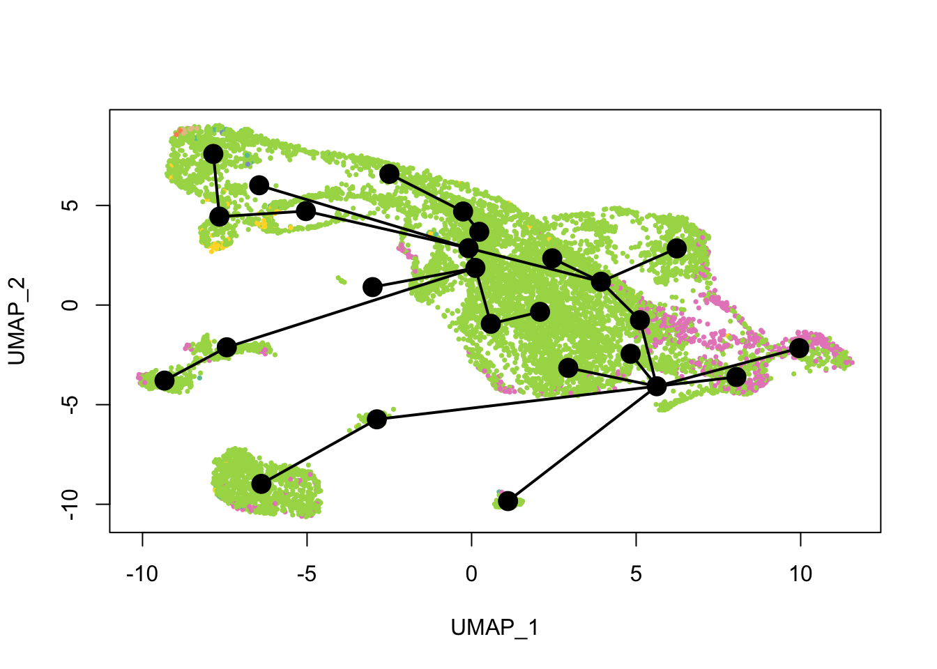

Past versions of lin1-1.png

Again, the qNSCs are the brown points near the top left, NPCs are green, and neurons are pink. It seems that multiple neural lineages formed. This is a much more complicated picture than the two branches of neurons projected on the first two PCs in the pseudotime figure in the kallisto | bustools paper (Supplementary Figure 6.5). It also seems that slingshot did not pick up the glial lineage (oligodendrocytes and astrocytes), as the vast majority of cells here are NPCs or neurons.

See how this looks with Leiden clusters.

plot(reducedDim(sds), col = cell_colors_clust, pch = 16, cex = 0.5)
lines(sds, lwd = 2, type = 'lineages', col = 'black')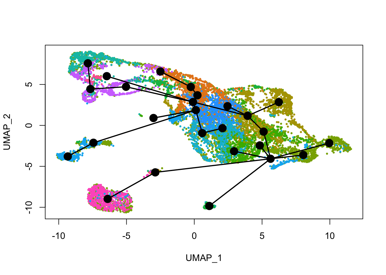

Past versions of lin2-1.png

Here slingshot thinks that somewhere around cluster 6 is a point where multiple neural lineages diverge. Different clustering (e.g. different random initiations of Louvain or Leiden algorithms) can lead to somewhat different trajectories, the the main structure is not affected. With different runs of Leiden clustering (without fixed seed), the branching point is placed in the region around its current location, near the small UMAP offshoot there.

Principal curves are smoothed representations of each lineage; pseudotime values are computed by projecting the cells onto the principal curves. What do the principal curves look like?

plot(reducedDim(sds), col = cell_colors, pch = 16, cex = 0.5)
lines(sds, lwd = 2, col = 'black')

Past versions of curves-1.png

Which cells are in which lineage? Here we plot the pseudotime values for each lineage.

nc <- 3
pt <- slingPseudotime(sds)
nms <- colnames(pt)
nr <- ceiling(length(nms)/nc)
pal <- viridis(100, end = 0.95)
par(mfrow = c(nr, nc))
for (i in nms) {
  colors <- pal[cut(pt[,i], breaks = 100)]
  plot(reducedDim(sds), col = colors, pch = 16, cex = 0.5, main = i)
  lines(sds, lwd = 2, col = 'black', type = 'lineages')
}

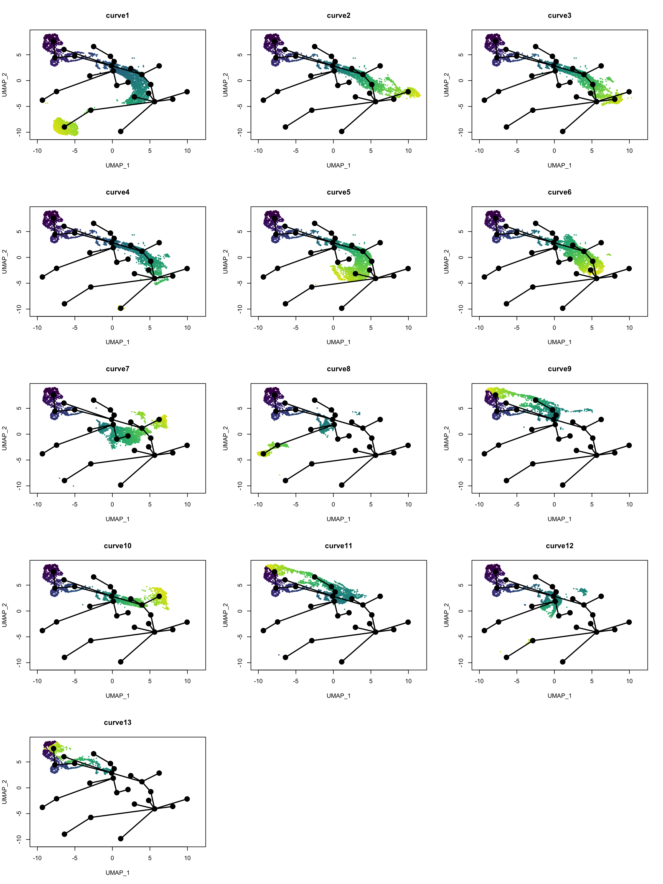
Past versions of pt-1.png

Some of the “lineages” seem spurious, especially those ending in clusters separated from the main lineage. Those may be distinct cell types of a different lineage from most cells mistaken by slingshot as highly differentiated cells from the same lineage, and SingleR does not have a reference that is detailed enough. Here manual cell type annotation with marker genes would be beneficial. Monocle 3 would have assigned disconnected trajectories to the separate clusters, but those clusters have been labeled NPCs or neurons, which must have come from neural stem cells. However, some lineages do seem reasonable, such as curves 2, 3, 5, and 7, going from qNSCs to neurons, though some lineages seem duplicated. Curves 9, 11, and 13 are saying that cell state goes back to the cluster with the qNSCs after a detour, though without more detailed manual cell type annotation, I don’t know what this means or if those “lineages” are real.

Running Slingshot on large datasets https://bioconductor.org/packages/release/bioc/vignettes/slingshot/inst/doc/vignette.html

For large datasets, we highgly recommend using the approx_points argument with slingshot (or getCurves). This allows the user to specify the resolution of the curves (ie. the number of unique points). While the MST construction operates on clusters, the process of iteratively projecting all points onto one or more curves may become computationally burdensome as the size of the dataset grows. For this reason, we set the default value for approx_points to either 150150 or the number of cells in the dataset, whichever is smaller. This should greatly ease the computational cost of exploratory analysis while having minimal impact on the resulting trajectories.

For maximally “dense” curves, set approx_points = FALSE, and the curves will have as many points as there are cells in the dataset. However, note that each projection step in the iterative curve-fitting process will now have a computational complexity proportional to n2�2 (where n� is the number of cells). In the presence of branching lineages, these dense curves will also affect the complexity of curve averaging and shrinkage.

We recommend a value of 100100-200200, hence the default value of 150150. Note that restricting the number of unique points along the curve does not impose a similar limit on the number of unique pseudotime values, as demonstrated below. Even with an unrealistically low value of 55 for approx_points, we still see a full color gradient from the pseudotime values:

sce5 <- slingshot(sce, clusterLabels = 'GMM', reducedDim = 'PCA',
                   approx_points = 5)

colors <- colorRampPalette(brewer.pal(11,'Spectral')[-6])(100)
plotcol <- colors[cut(sce5$slingPseudotime_1, breaks=100)]

plot(reducedDims(sce5)$PCA, col = plotcol, pch=16, asp = 1)
lines(SlingshotDataSet(sce5), lwd=2, col='black')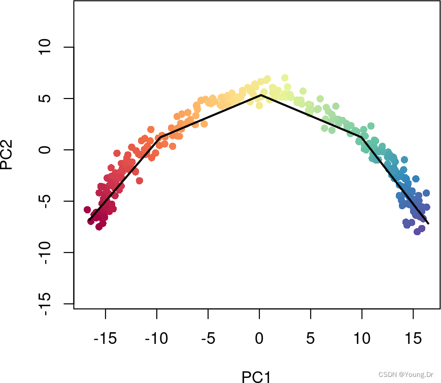

Multiple Trajectories

In some cases, we are interested in identifying multiple, disjoint trajectories. Slingshot handles this problem in the initial MST construction by introducing an artificial cluster, called omega. This artificial cluster is separated from every real cluster by a fixed length, meaning that the maximum distance between any two real clusters is twice this length. Practically, this sets a limit on the maximum edge length allowable in the MST. Setting omega = TRUE will implement a rule of thumb whereby the maximum allowable edge length is equal to 33 times the median edge length of the MST constructed without the artificial cluster (note: this is equivalent to saying that the default value for omega_scale is 1.51.5).

rd2 <- rbind(rd, cbind(rd[,2]-12, rd[,1]-6))
cl2 <- c(cl, cl + 10)
pto2 <- slingshot(rd2, cl2, omega = TRUE, start.clus = c(1,11))

plot(rd2, pch=16, asp = 1,
     col = c(brewer.pal(9,"Set1"), brewer.pal(8,"Set2"))[cl2])
lines(SlingshotDataSet(pto2), type = 'l', lwd=2, col='black')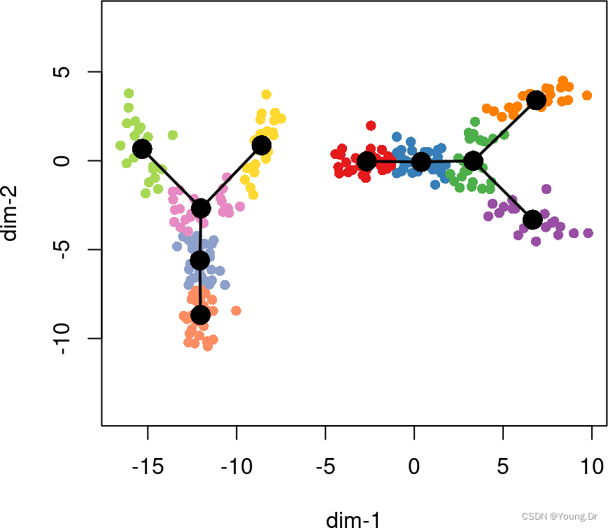

After fitting the MST, slingshot proceeds to fit simultaneous principal curves as usual, with each trajectory being handled separately.

plot(rd2, pch=16, asp = 1,
     col = c(brewer.pal(9,"Set1"), brewer.pal(8,"Set2"))[cl2])
lines(SlingshotDataSet(pto2), lwd=2, col='black')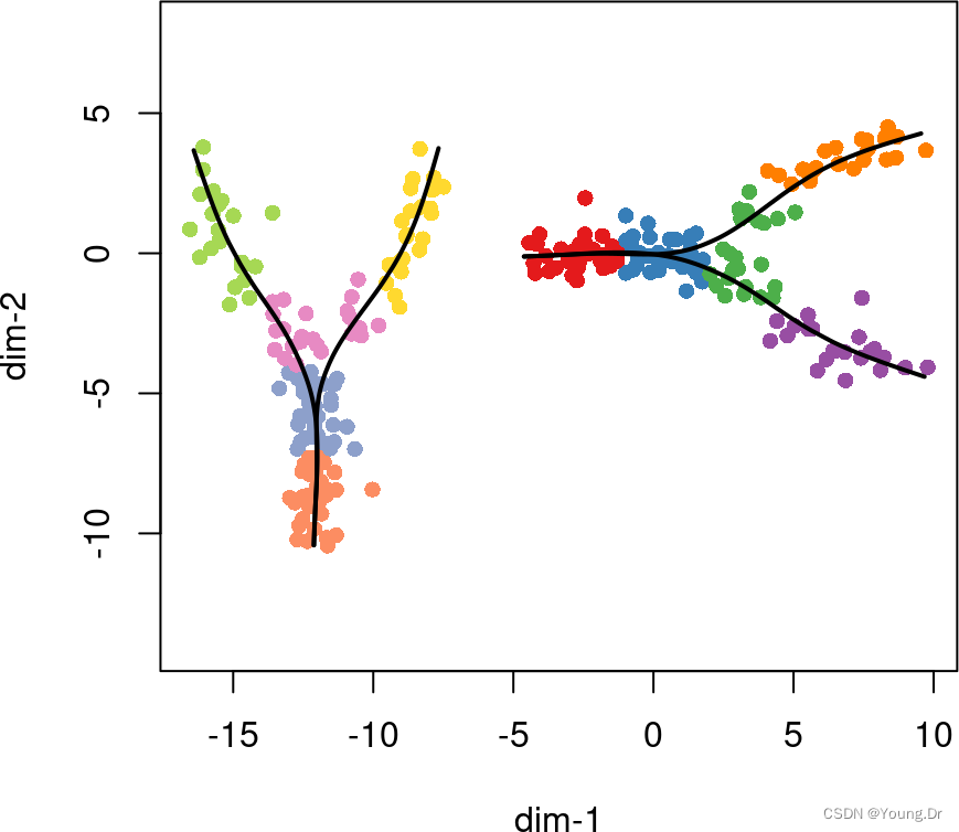

5.5Projecting Cells onto Existing Trajectories

Sometimes, we may want to use only a subset of the cells to determine a trajectory, or we may get new data that we want to project onto an existing trajectory. In either case, we will need a way to determine the positions of new cells along a previously constructed trajectory. For this, we can use the predict function (since this function is not native to slingshot, see ?`predict,PseudotimeOrdering-method` for documentation).

# our original PseudotimeOrdering
pto <- sce$slingshot

# simulate new cells in PCA space
newPCA <- reducedDim(sce, 'PCA') + rnorm(2*ncol(sce), sd = 2)

# project onto trajectory
newPTO <- slingshot::predict(pto, newPCA)

This will yield a new, hybrid object with the trajectories (curves) from the original data, but the pseudotime values and weights for the new cells. For reference, the original cells are shown in grey below, but they are not included in the output from predict.

newplotcol <- colors[cut(slingPseudotime(newPTO)[,1], breaks=100)]
plot(reducedDims(sce)$PCA, col = 'grey', bg = 'grey', pch=21, asp = 1,
     xlim = range(newPCA[,1]), ylim = range(newPCA[,2]))
lines(SlingshotDataSet(sce), lwd=2, col = 'black')
points(slingReducedDim(newPTO), col = newplotcol, pch = 16)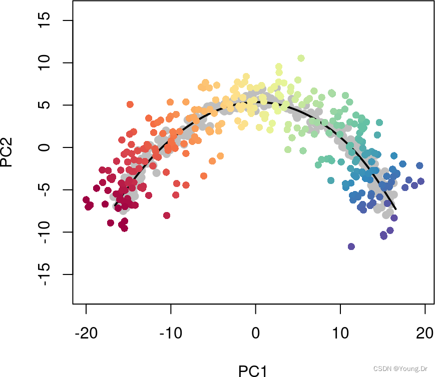

Differential expression

Let’s look at which genes are differentially expressed along one of those lineages (linage 2). In dynverse, feature (gene) importance is calculated by using gene expression to predict pseudotime value with random forest and finding genes that contribute the most to the accuracy of the response. Since it’s really not straightforward to convert existing pseudotime results to dynverse format, it would be easier to build a random forest model. Variable importance will be calculated for the top 300 highly variable genes here, with tidymodels. This is to make the code run faster. There are other methods of trajectory DE as well, which may be more appropriate but more time consuming to run, such as tradeSeq and SpatialDE (when run with one dimension).

# Get top highly variable genes
top_hvg <- HVFInfo(seu) %>% 
  mutate(., bc = rownames(.)) %>% 
  arrange(desc(residual_variance)) %>% 
  top_n(300, residual_variance) %>% 
  pull(bc)
# Prepare data for random forest
dat_use <- t(GetAssayData(seu, slot = "data")[top_hvg,])
dat_use_df <- cbind(slingPseudotime(sds)[,2], dat_use) # Do curve 2, so 2nd columnn
colnames(dat_use_df)[1] <- "pseudotime"
dat_use_df <- as.data.frame(dat_use_df[!is.na(dat_use_df[,1]),])

The subset of data is randomly split into training and validation; the model fitted on the training set will be evaluated on the validation set.

dat_split <- initial_split(dat_use_df)
dat_train <- training(dat_split)
dat_val <- testing(dat_split)

tidymodels is a unified interface to different machine learning models, a “tidier” version of caret. The code chunk below can easily be adjusted to use other random forest packages as the back end, so no need to learn new syntax for those packages.

model <- rand_forest(mtry = 200, trees = 1400, min_n = 15, mode = "regression") %>%
  set_engine("ranger", importance = "impurity", num.threads = 3) %>%
  fit(pseudotime ~ ., data = dat_train)

The model is evaluated on the validation set with 3 metrics: room mean squared error (RMSE), coefficient of determination using correlation (rsq, between 0 and 1), and mean absolute error (MAE).

val_results <- dat_val %>% 
  mutate(estimate = predict(model, .[,-1]) %>% pull()) %>% 
  select(truth = pseudotime, estimate)
metrics(data = val_results, truth, estimate)

#> # A tibble: 3 x 3
#>   .metric .estimator .estimate
#>   <chr>   <chr>          <dbl>
#> 1 rmse    standard       1.47 
#> 2 rsq     standard       0.962
#> 3 mae     standard       0.739

RMSE and MAE should have the same unit as the data. As pseudotime values here usually have values much larger than 2, the error isn’t too bad. Correlation (rsq) between slingshot’s pseudotime and random forest’s prediction is very high, also showing good prediction from the top 300 highly variable genes.

summary(dat_use_df$pseudotime)

#>    Min. 1st Qu.  Median    Mean 3rd Qu.    Max. 
#>   0.000   4.172  13.385  11.914  18.177  24.116

Now it’s time to plot some genes deemed the most important to predicting pseudotime:

var_imp <- sort(model$fit$variable.importance, decreasing = TRUE)
top_genes <- names(var_imp)[1:6]
# Convert to gene symbol
top_gene_name <- gns$gene_name[match(top_genes, gns$gene)]

par(mfrow = c(3, 2))
for (i in seq_along(top_genes)) {
  colors <- pal[cut(dat_use[,top_genes[i]], breaks = 100)]
  plot(reducedDim(sds), col = colors, 
       pch = 16, cex = 0.5, main = top_gene_name[i])
  lines(sds, lwd = 2, col = 'black', type = 'lineages')
}

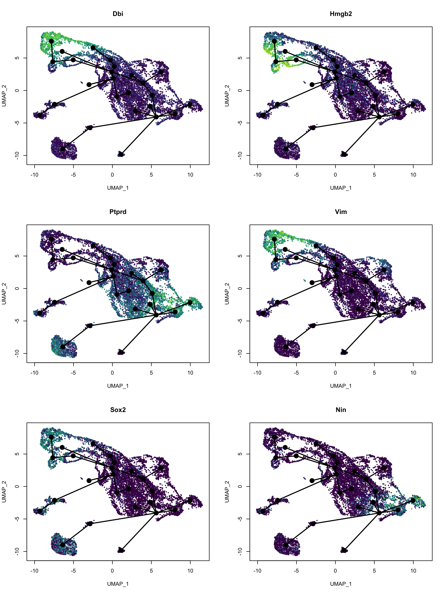
Past versions of genes-1.png

These genes do highlight different parts of the trajectory. A quick search on PubMed did show relevance of these genes to development of the central nervous system in mice.