


👨🎓个人主页
💥💥💞💞欢迎来到本博客❤️❤️💥💥
🏆博主优势:🌞🌞🌞博客内容尽量做到思维缜密,逻辑清晰,为了方便读者。
⛳️座右铭:行百里者,半于九十。
📋📋📋本文目录如下:🎁🎁🎁
目录
💥1 概述
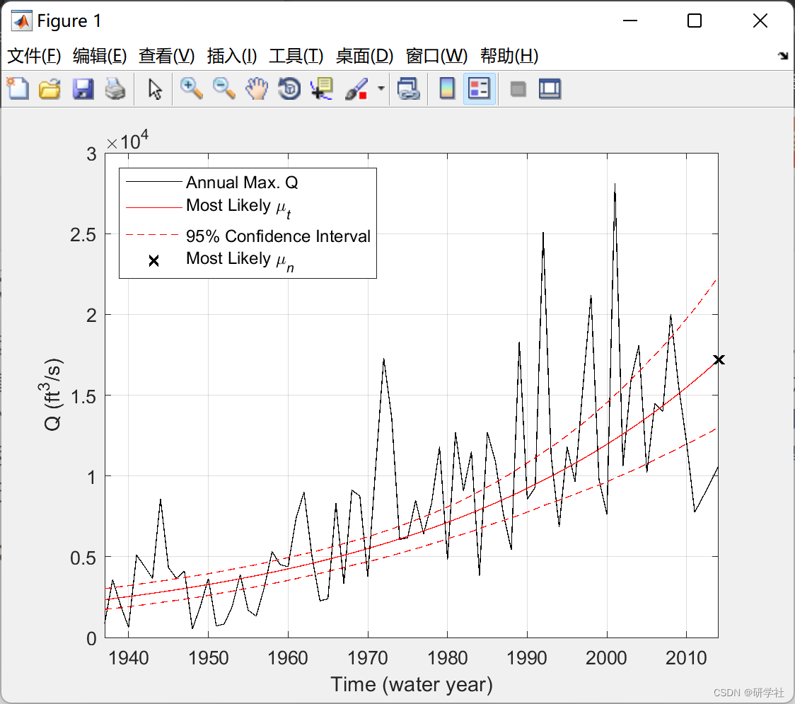
在 NS 模型中,LPIII 分布的均值随时间变化。返回周期不是在真正的非平稳意义上计算的,而是针对平均值的固定值计算的。换句话说,假设分布在时间上保持固定,则计算返回周期。默认情况下,在对 NS LPIII 模型参数的估计值应用 bayes_LPIII时,将计算并显示更新的 ST 返回周期。更新的 ST 返回周期是通过计算与拟合期结束时的 NS 均值或 t = t(end) 相关的回报期获得的,假设分布在记录结束后的时间保持固定。
一、研究背景与意义
在自然灾害预测、水资源管理和电力系统等领域,对极端事件的准确预测至关重要。峰值放电作为极端气候事件的一种表现形式,其发生频率和强度对于评估灾害风险和制定应对策略具有重要意义。本研究旨在通过贝叶斯推理方法,对稳态(ST)和非稳态(NS)LPIII模型进行参数估计,以更好地拟合峰值放电数据,提高预测精度。
二、理论基础
- 贝叶斯推理:贝叶斯推理是一种基于概率的统计方法,通过结合先验信息和样本数据来更新对未知参数的认识。在贝叶斯框架下,参数被视为随机变量,其后验分布反映了在给定数据下参数的不确定性。
- LPIII模型:LPIII模型是一种用于描述极端气候事件(如峰值放电)的统计模型。在稳态(ST)情况下,模型的参数是固定的;而在非稳态(NS)情况下,模型的参数会随时间发生变化。
三、研究方法
- 数据收集与预处理:收集峰值放电数据,并进行预处理,包括数据清洗、缺失值处理、异常值检测等。
- 模型构建:根据LPIII模型的定义,分别构建稳态(ST)和非稳态(NS)两种情况下的模型。在NS模型中,需要引入时间相关的参数来描述均值的变化。
- 贝叶斯推理:利用贝叶斯公式,结合先验分布和似然函数,计算参数的后验分布。通过MCMC(马尔可夫链蒙特卡洛)方法,如DREAM_ZS算法,对后验分布进行采样,以获得参数的估计值。
- 模型评估:通过比较模型的拟合效果(如均方误差、赤池信息准则等)和预测性能(如返回周期、返回水平等),评估稳态(ST)和非稳态(NS)LPIII模型的优劣。
四、研究结果
- 参数估计:利用贝叶斯推理方法,得到了稳态(ST)和非稳态(NS)LPIII模型的参数估计值。在NS模型中,参数随时间的变化趋势得到了明确的描述。
- 模型拟合效果:通过对比稳态(ST)和非稳态(NS)模型的拟合效果,发现NS模型能够更好地捕捉峰值放电数据的动态变化特征。
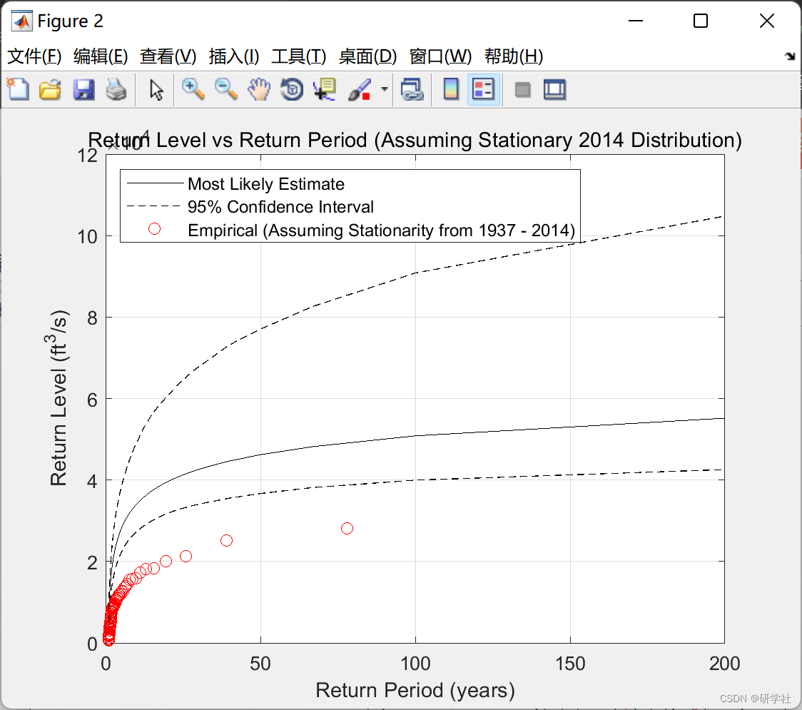
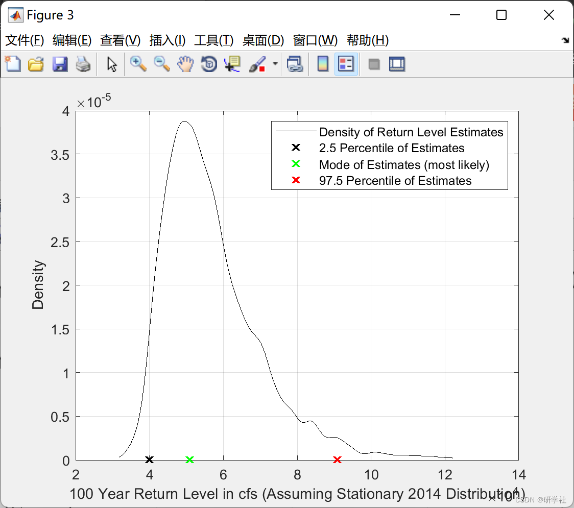
- 预测性能:基于得到的模型参数,对峰值放电的返回周期和返回水平进行了预测。结果显示,NS模型的预测性能优于ST模型,尤其是在长期预测方面。
五、结论与展望
本研究通过贝叶斯推理方法,成功估计了稳态(ST)和非稳态(NS)LPIII模型的参数,并发现NS模型在拟合峰值放电数据方面具有显著优势。未来研究可以进一步探索其他类型的非稳态模型,以及如何将贝叶斯推理与其他机器学习算法相结合,以提高极端气候事件的预测精度和鲁棒性。
📚2 运行结果
部分代码:
cf = 1; %multiplication factor to convert input Q to ft^3/s
Mj = 2; %1 for ST LPIII, 2 for NS LPIII with linear trend in mu
y_r = 0; %Regional estimate of gamma (skew coefficient)
SD_yr = 0.55; %Standard deviation of the regional estimate
%Prior distributions (input MATLAB abbreviation of distribution name used in
%function call, i.e 'norm' for normal distribution as in 'normpdf')
marg_prior{1,1} = 'norm';
marg_prior{1,2} = 'unif';
marg_prior{1,3} = 'unif';
marg_prior{1,4} = 'unif';
%Hyper-parameters of prior distributions (input in order of use with
%function call, i.e [mu, sigma] for normpdf(mu,sigma))
marg_par(:,1) = [y_r, SD_yr]'; %mean and std of informative prior on gamma
marg_par(:,2) = [0, 6]'; %lower and upper bound of uniform prior on scale
marg_par(:,3) = [-10, 10]'; %lower and upper bound of uniform prior on location
marg_par(:,4) = [-0.15, 0.15]'; %lower and upper bound of uniform prior on trend
%DREAM_(ZS) Variables
if Mj == 1; d = 3; end %define number of parameters based on model
if Mj == 2; d = 4; end
N = 3; %number of Markov chains
T = 8000; %number of generations
%create function to initialize from prior
prior_draw = @(r,d)prior_rnd(r,d,marg_prior,marg_par);
%create function to compute prior density
prior_density = @(params)prior_pdf(params,d,marg_prior,marg_par);
%create function to compute unnormalized posterior density
post_density = @(params)post_pdf(params,data,cf,Mj,prior_density);
%call the DREAM_ZS algorithm
%Markov chains | post. density | archive of past states
[x, p_x, Z] = dream_zs(prior_draw,post_density,N,T,d,marg_prior,marg_par);
%% Post Processing and Figures
%options:
%Which mu_t for calculating return level vs. return period? (don't change
%for estimates corresponding ti distribution at end of record, or updated ST distribution)
t = data(:,1) - min(data(:,1)); %time (in years from the start of the fitting period)
idx_mu_n = size(t,1); %calculates and plots RL vs RP for mu_t associated with t(idx_mu_n)
%(idx_mu_n = size(t,1) for uST distribution)
%Which return level for denisty plot?
sRP = 100; %plots density of return level estimates for this return period
%Which return periods for output table? %outputs table of return level estimates for these return periods
RP_out =[200; 100; 50; 25; 10; 5; 2];
%end options
%apply burn in (use only half of each chain) and rearrange chains to one sample
x1 = x(round(T/2)+1:end,:,:); %burn in
p_x1 = p_x(round(T/2)+1:end,:,:);
post_sample = reshape(permute(x1,[1 3 2]),size(x1,1)*N,d,1); %columns are marginal posterior samples
sample_density = reshape(p_x1,size(p_x1,1)*N,1); %corresponding unnormalized density
%find MAP estimate of theta
idx_theta_MAP = max(find(sample_density == max(sample_density)));
theta_MAP = post_sample(idx_theta_MAP,:); %most likely parameter estimate
%Compute mu as a function of time and credible intervals
if Mj == 1; mu_t = repmat(post_sample(:,3),1,length(t));end %ST model, mu is constant
if Mj == 2; mu_t = repmat(post_sample(:,3),1,length(t)) + post_sample(:,4)*t';end %NS mu = f(t)
MAP_mu_t = mu_t(idx_theta_MAP,:); %most likely estimate of the location parameter
low_mu_t = prctile(mu_t,2.5,1); %2.5 percentile of location parameter
high_mu_t = prctile(mu_t,97.5,1); %97.5 percentile of location parameter
%compute quantiles of the LPIII distribution
p = 0.01:0.005:0.995; %1st - 99.5th quantile (1 - 200 year RP)
a=1;
RLs = nan(size(post_sample,1),size(p,2));
for i = 1:size(post_sample,1); %compute return levels for each posterior sample
RLs(i,:) = lp3inv(p,post_sample(i,1),post_sample(i,2),mu_t(i,idx_mu_n));
a = a+1;
if a == round(size(post_sample,1)/10) || i == size(post_sample,1);
clc
disp(['Calculating Return Levels ' num2str(round(i/size(post_sample,1)*100)) '% complete'])
a = 1;
end
end
MAP_RL = RLs(idx_theta_MAP,:); %Return levels associated with most likely parameter estimate
low_RL = prctile(RLs,2.5,1); %2.5 percentile of return level estimates
high_RL = prctile(RLs,97.5,1); %97.5 percentile of return level estimates
🎉3 参考文献
部分理论来源于网络,如有侵权请联系删除。
[1]吴英捷.基于参数时变离散DBN的无人机决策参数估计与学习方法研究[J].[2024-10-16].
[2]孙丙香,高科,姜久春,等.基于ANFIS和减法聚类的动力电池放电峰值功率预测[J].电工技术学报, 2015, 30(004):272-280.DOI:10.3969/j.issn.1000-6753.2015.04.034.
[3]杨洁,刘尚合,国海广,等.集成电路静电放电电压与注入能量的相关性研究[C]//中国物理学会静电专业委员会第十二届学术年会论文集.2005.


 295
295

 被折叠的 条评论
为什么被折叠?
被折叠的 条评论
为什么被折叠?
 到【灌水乐园】发言


