10X单细胞（10X空间转录组）转录因子活性分析之DoRothEA

hello，大家好，今天给大家分享一个转录因子活性预测的工具，DoRothEA，在多篇高分文章中都有运用，我们就来看看这个软件的优势吧。大家可以参考DoRothEA。

先来看看介绍

首先是数据库，DoRothEA是一种包含转录因子（TF）与其靶标相互作用的基因集。一个TF及其对应靶点的集合被定义为调节子（regulons）。DoRothEA regulons 收集了文献，ChIP-seq peaks，TF结合位点基序，从基因表达推断相互作用等不同类型的互作证据。TF和靶标之间的互作可信度根据支持的证据数量划分为A-E五个等级，A是最可信，E为可信度低。

TF 活性是根据其靶标的 mRNA 表达水平计算的。 因此，可以将 TF 活性视为给定转录状态的代表 。

看一看代码案例

安装和加载

if (!requireNamespace("BiocManager", quietly = TRUE))
    install.packages("BiocManager")

BiocManager::install("dorothea")
## We load the required packages
library(dorothea)
library(dplyr)
library(Seurat)
library(tibble)
library(pheatmap)
library(tidyr)
library(viper)

读取数据(以pbmc为例)

## Load the PBMC dataset
pbmc.data <- Read10X(data.dir = "filtered_gene_bc_matrices/hg19/")

## Initialize the Seurat object with the raw (non-normalized data).
pbmc <- CreateSeuratObject(counts = pbmc.data, project = "pbmc3k", 
                           min.cells = 3, min.features = 200)

前处理（可选，如果读取的rds已经做过处理，这一步就不需要了）

## Identification of mithocondrial genes
pbmc[["percent.mt"]] <- PercentageFeatureSet(pbmc, pattern = "^MT-")

## Filtering cells following standard QC criteria.
pbmc <- subset(pbmc, subset = nFeature_RNA > 200 & nFeature_RNA < 2500 & 
    percent.mt < 5)

## Normalizing the data
pbmc <- NormalizeData(pbmc, normalization.method = "LogNormalize", 
    scale.factor = 10000)

pbmc <- NormalizeData(pbmc)

## Identify the 2000 most highly variable genes
pbmc <- FindVariableFeatures(pbmc, selection.method = "vst", nfeatures = 2000)

## In addition we scale the data
all.genes <- rownames(pbmc)
pbmc <- ScaleData(pbmc, features = all.genes)

降维聚类（可选，Seurat的方法，通常我们前面都已经分析过了）

pbmc <- RunPCA(pbmc, features = VariableFeatures(object = pbmc), 
               verbose = FALSE)
pbmc <- FindNeighbors(pbmc, dims = 1:10, verbose = FALSE)
pbmc <- FindClusters(pbmc, resolution = 0.5, verbose = FALSE)
pbmc <- RunUMAP(pbmc, dims = 1:10, umap.method = "uwot", metric = "cosine")

pbmc.markers <- FindAllMarkers(pbmc, only.pos = TRUE, min.pct = 0.25, 
                               logfc.threshold = 0.25, verbose = FALSE)

## Assigning cell type identity to clusters
new.cluster.ids <- c("Naive CD4 T", "Memory CD4 T", "CD14+ Mono", "B", "CD8 T",
                     "FCGR3A+ Mono", "NK", "DC", "Platelet")
names(new.cluster.ids) <- levels(pbmc)
pbmc <- RenameIdents(pbmc, new.cluster.ids)
DimPlot(pbmc, reduction = "umap", label = TRUE, pt.size = 0.5) + NoLegend()

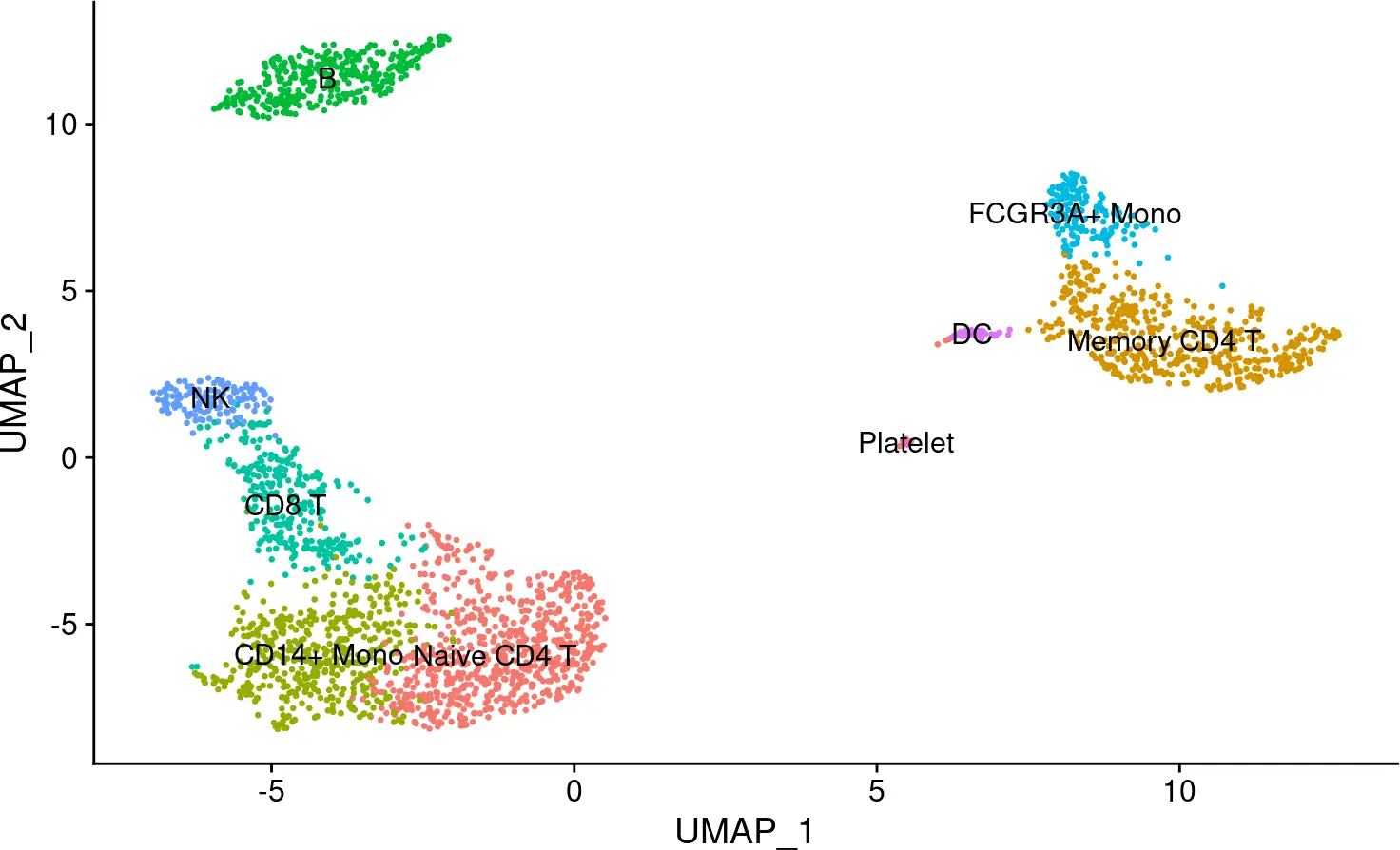
图片.png

计算细胞的TF活性,案例中首先通过使用包装函数 run_viper() 在 DoRothEA 的regulons上运行 VIPER 以获得 TFs activity。 该函数可以处理不同的输入类型，例如矩阵、数据框、表达式集甚至 Seurat 对象。 在 seurat 对象的情况下，该函数返回相同的 seurat 对象，其中包含一个名为 dorothea 的assay，其中包含slot数据中的 TFs activity。

## We read Dorothea Regulons for Human:
dorothea_regulon_human <- get(data("dorothea_hs", package = "dorothea"))

## We obtain the regulons based on interactions with confidence level A, B and C
regulon <- dorothea_regulon_human %>%
    dplyr::filter(confidence %in% c("A","B","C"))

## We compute Viper Scores 
pbmc <- run_viper(pbmc, regulon,
                  options = list(method = "scale", minsize = 4, 
                                 eset.filter = FALSE, cores = 1, 
                                 verbose = FALSE))

然后我们应用 Seurat 按照与上述相同的方法但使用 TFs activity分数对细胞进行聚类。

## We compute the Nearest Neighbours to perform cluster
DefaultAssay(object = pbmc) <- "dorothea"
pbmc <- ScaleData(pbmc)
pbmc <- RunPCA(pbmc, features = rownames(pbmc), verbose = FALSE)
pbmc <- FindNeighbors(pbmc, dims = 1:10, verbose = FALSE)
pbmc <- FindClusters(pbmc, resolution = 0.5, verbose = FALSE)

pbmc <- RunUMAP(pbmc, dims = 1:10, umap.method = "uwot", metric = "cosine")

pbmc.markers <- FindAllMarkers(pbmc, only.pos = TRUE, min.pct = 0.25, 
                               logfc.threshold = 0.25, verbose = FALSE)

## Assigning cell type identity to clusters
new.cluster.ids <- c("Naive CD4 T", "Memory CD4 T", "CD14+ Mono", "B", "CD8 T", 
                     "FCGR3A+ Mono", "NK", "DC", "Platelet")
names(new.cluster.ids) <- levels(pbmc)
pbmc <- RenameIdents(pbmc, new.cluster.ids)
DimPlot(pbmc, reduction = "umap", label = TRUE, pt.size = 0.5) + NoLegend()

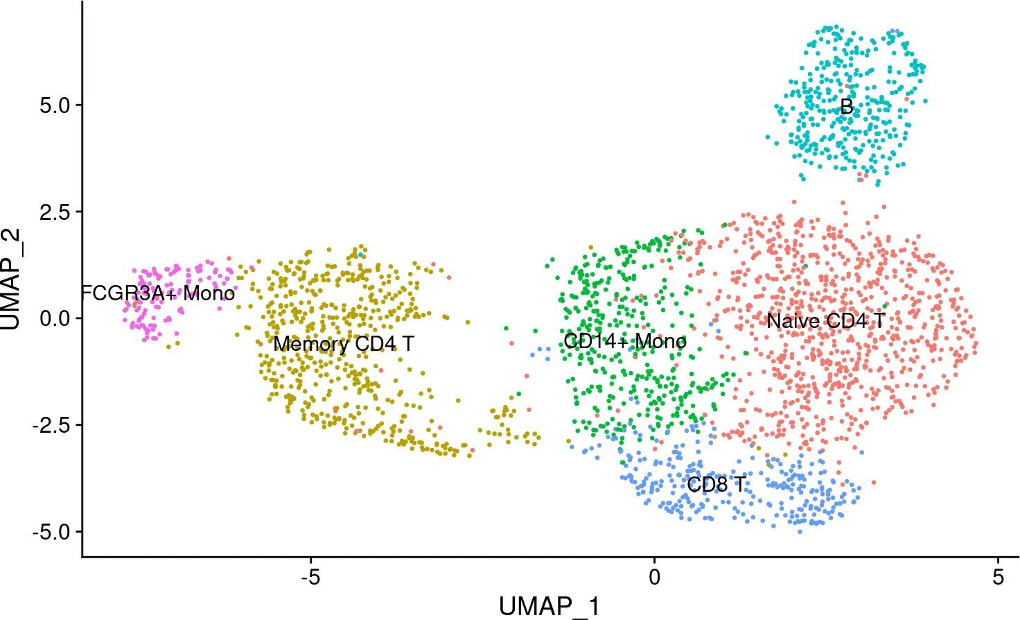
图片.png

每个细胞群的TF活性（相当于每个细胞群的bulk RNAseq）,根据先前计算的 DoRothEA regulons的 VIPER 分数，我们根据它们的TF activities来表征不同的细胞群。

## We transform Viper scores, scaled by seurat, into a data frame to better 
## handling the results
viper_scores_df <- GetAssayData(pbmc, slot = "scale.data", 
                                    assay = "dorothea") %>%
  data.frame(check.names = F) %>%
  t()

## We create a data frame containing the cells and their clusters
CellsClusters <- data.frame(cell = names(Idents(pbmc)), 
                            cell_type = as.character(Idents(pbmc)),
                            check.names = F)

## We create a data frame with the Viper score per cell and its clusters
viper_scores_clusters <- viper_scores_df  %>%
  data.frame() %>% 
  rownames_to_column("cell") %>%
  gather(tf, activity, -cell) %>%
  inner_join(CellsClusters)

## We summarize the Viper scores by cellpopulation
summarized_viper_scores <- viper_scores_clusters %>% 
  group_by(tf, cell_type) %>%
  summarise(avg = mean(activity),
            std = sd(activity))

选择在细胞群间变化最大的20个TFs进行可视化

## We select the 20 most variable TFs. (20*9 populations = 180)
highly_variable_tfs <- summarized_viper_scores %>%
  group_by(tf) %>%
  mutate(var = var(avg))  %>%
  ungroup() %>%
  top_n(180, var) %>%
  distinct(tf)

## We prepare the data for the plot
summarized_viper_scores_df <- summarized_viper_scores %>%
  semi_join(highly_variable_tfs, by = "tf") %>%
  dplyr::select(-std) %>%   
  spread(tf, avg) %>%
  data.frame(row.names = 1, check.names = FALSE) 
palette_length = 100
my_color = colorRampPalette(c("Darkblue", "white","red"))(palette_length)

my_breaks <- c(seq(min(summarized_viper_scores_df), 0, 
                   length.out=ceiling(palette_length/2) + 1),
               seq(max(summarized_viper_scores_df)/palette_length, 
                   max(summarized_viper_scores_df), 
                   length.out=floor(palette_length/2)))

viper_hmap <- pheatmap(t(summarized_viper_scores_df),fontsize=14, 
                       fontsize_row = 10, 
                       color=my_color, breaks = my_breaks, 
                       main = "DoRothEA (ABC)", angle_col = 45,
                       treeheight_col = 0,  border_color = NA) 

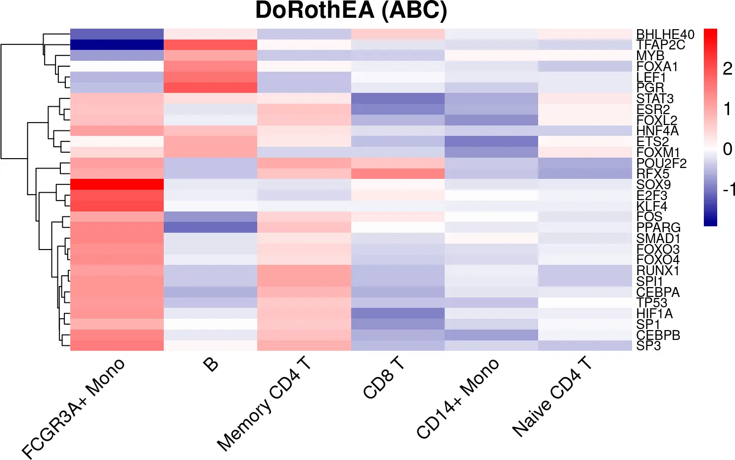
图片.png

感觉还挺好，方便，能说明一些生物学的问题

生活很好，有你更好