Microfacet Models for Refraction through Rough Surfaces

最新推荐文章于 2024-09-03 12:14:31 发布

wodownload2

最新推荐文章于 2024-09-03 12:14:31 发布

阅读量904

点赞数

分类专栏： opengl 文章标签： BRDF

本文链接：https://blog.csdn.net/wodownload2/article/details/100084678

版权

opengl 专栏收录该内容

60 篇文章

订阅专栏

https://www.cs.cornell.edu/~srm/publications/EGSR07-btdf.pdf
http://www.codinglabs.net/article_physically_based_rendering_cook_torrance.aspx

microfacet models were introduced to graphics by cook and torrance, based on earlier work from optic, to model light direction from rough surfaces. many variations have been proposed. microfacet models are widely used in graphics and have proven effective in modeling many real surfaces.

microfacet theory
a BSDF (bidirectional scattering distribution function) describes how light scatters from a surface. it is defined as the ratio of scatterd radiance 辐射率 in a direction o caused per unit irradiance 辐照度 incident from direction i, and we will denote it as fs(i,o,n) to emphasize its dependence on the local surface normal n. if restricted to only reflection or transmission, it is often called the BRDF or BTDF, respectively, and our BSDF will be the sum of a BRDF, fr, and a BTDF, ft , term.
since we want to include both reflection and transmission, we will take care of our derivations and equations can correctly handle directions on either side of the surface.

in microfacet models, a detailed microsurface is replaced by a simplified macrosurface (see figure 4)
在这里插入图片描述
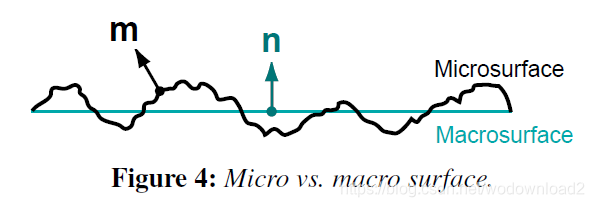
with a modified scattering function (BSDF) that matches the aggregate directional scattering of the microsurface (i.e. both should appear the same from a distance). this assumes that microsurface detail is too small to be seen directly, so only the far-field directional scattering pattern matters. Typically geometric optics is assumed and only single scattering is modeled, to simplify the problem. Wave effects and light that strikes the surface twice (or more) are ignored or must be handled separately.

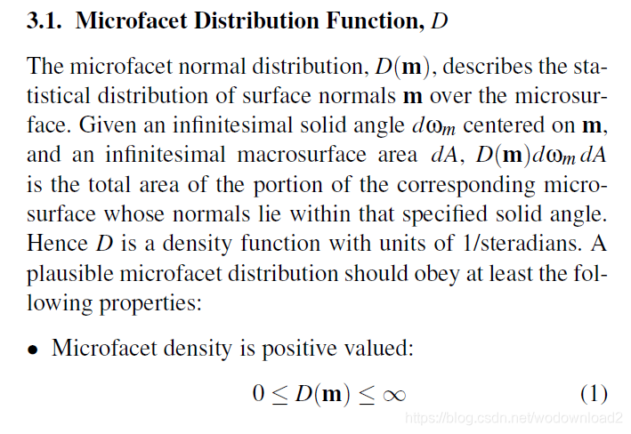
Rather than working with a particular micro-surface configuration, it is assumed that the microsurface can be adequately
described by two statistical measures, a microfacet distribution function D and a shadowing-masking function G, together with a microsurface BSDF f m s . .

在这里插入图片描述

macrosurface BRDF integral
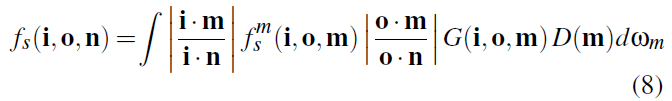
the macrosurface BSDF is designed to match the aggregate directional (single) scattering behabiour of the microsurface. we can compute it by intergrating (i.e. summing) the (i.e. summing) the contributions over all visible corresponding parts of the microsurface, each of which scatters light according to the microsurface’s BSDF, 在这里插入图片描述

the product of the D and G gives the corresponding visible area of the microsurface for each micronormal m. We also need to apply correction factors to first transform incident irradiance onto the microsurface and then transform the scattered radiance back to the macrosurface, because both irradiance and radiance are measured relative to a surface’s projected area. The resulting integral for
the macrosurface BSDF is:
在这里插入图片描述

在这里插入图片描述

以下
https://zhuanlan.zhihu.com/p/20119162
最常用的microfacet模型是cook torrance。与普通的着色模型的区别在于，普通的着色模型假设着色的区域是一个平滑的表面，表面的方向可以用一个单一的法向量来定义。而microfacet模型则认为：
1、着色的区域是一个无数比入射光线覆盖范围更小的微小表面组成的粗糙区域。
2、所有这些微小表面都是光滑镜面反射的表面。
因为这种模型认为着色区域的表面是由无数方向不同的小表面组成的，所以在microfacet模型中，着色区域并不能用一个法线来表示表面的方向，只能用一个概率分布函数D来计算任意方向的微小表面在着色区域中存在的概率。

因为每个微小表面都做完美镜面反射，完美镜面反射只在入射光和反射光根据法线镜面反射对称的时候才有能量，所以在计算微小表面的BRDF值时，只用先根据入射方向wi和出射方向wo计算出中间向量wm，也就是微小表面的法线方向，然后就可以用法线分布函数计算出这个能够完美镜面反射当前入射和出射光D(wm)。
同样因为是完美镜面反射的缘故，cook-torrance模型的另一个因素就是菲涅尔（fresnel）项F(wi,wm)，这个项用于计算不同入射角度的情况下反射的光线的强度，对于导体和电机、介质记得使用不同的fresnel公式。最后，为了更好的模拟着色区域的凹凸不平，G(wi,wo,wm)项则模拟了凹凸表面间的遮挡因素。省略掉复杂具体的推导过程，Cook Torrance模型的BRDF就是：

在这里插入图片描述
其中
是微小表面的法线，就是入射和出射光线中间的方向，wn是着色区域实际表面的法线，和普通着色模型中的法线是一样的。

人们也根据这种模型设计出了许多不一样的法线分布函数D。大家熟知的blinn-phong就是一种很简单的分布函数，相信大家在学简单的lighting shader的时候，肯定看到过这段代码：

// 计算镜面反射强度
float NdotH = dot(normal, Wm); // Wm = normalize(Wo + Wi)
float specularIntensity = pow(saturate( NdotH ), e);

这就是基于blinn-phong的法线分布
在这里插入图片描述，其中e代表粗糙程度。
blinn-phong并不是一个非常真实的分布，上面的公式也并不满足能量守恒定律。（D需要满足wm在半球面上积分为1，Blinn-Phong还需乘以一个常量才满足这个条件）。

近年来有许多新的分布函数被发明处理例如beckmann, ggx等，他们的能量分布都更接近光学仪器测量的反射数据。
disney brdf也使用了ggx分布。本文后面的所有渲染结果也使用了ggx。G项也有各种不同的选择，本文使用了有粗糙度作为参数的smith模型。网上ggx和smith g项的实现很多。

粗糙镜面反射
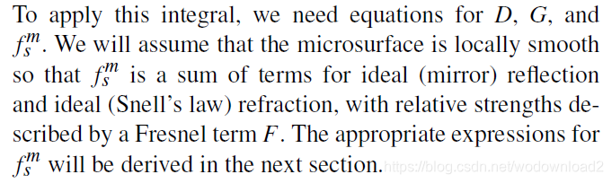
有了microfacet，我们就可以模拟现实中由非常细小的粗糙表面组成的镜面反射了。生活中这种材质很常见，各种粗糙的金属，iPhone6的背面也是：
在这里插入图片描述
这种材质将入射光根据表面的粗糙程度分散的反射到镜面反射方向周围的方向，表面越粗糙反射的分布越分散。

下面的两张渲染结果都是用GGX分布计算的，第二张比第一张更加粗糙（个人觉得第二张很像深空灰iPhone6）。
在这里插入图片描述

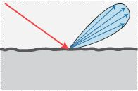
粗糙镜面折射
microfacet模型同样可用于模拟粗糙的折射表面。顾名思义这一种材质则会将入射光线同时反射和折射到镜面反射和折射周围的方向，分布大小取决于表面的粗糙程度。
在这里插入图片描述
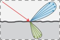
这种材质在现实中的例子就是各种毛玻璃：

在BRDF计算的时候先根据入射的方向决定当前发生的是反射还是折射，然后用不同的方法算出两种情况下的wm，然后再用反射或者折射的microfacet公式计算出结果。简单写一下这个过程的伪代码：

float f(Vector3 wo, Vector3 wi, Vector3 wn)
{
	bool IsReflection = true;
	// 根据出入射方向和法线方向判定是反射还是折射
	if(Dot(wo, wn) * Dot(wi, wn) < 0.0f)
		IsReflection = false;

	Vector3 wm;
	if(IsReflection)
		wm = Normalize(wo + wi);
	else // 如果是折射则根据折射率算出wm
		wm = -Normalize(etai * wo + etat * wi);

	float D = GGX_D(wm, Roughness);
	float F = Fresnel(Dot(wo, wm), etai, etat);
	float G = GGX_G(wo, wi, wm, Roughness);

	// 有力D，F和G就可以套入Microfacet的公式计算当前BRDF的返回值。
}

多层材质（multi-layered material）
现实中其实绝大多数的材质都有超过一层以上的组成部分，例如木地板。木头本身是粗糙的漫反射表面，但是木地板都会在表面上涂上一层镜面反射的透明油漆。这一类的材质比比皆是，塑料，大理石，瓷器等等。而且严格来说许多漫反射的材质都有些许的镜面反射的组成部分在里面。这大概也是当年最早的固定渲染管线可以让你设置镜面光和漫反射光的颜色，渲染的结果就像塑料一样的原因吧。
在这里插入图片描述
所以想要渲染出上图一样的材质，就也一定要在构建材质模型的时候考虑多层的信息。幸运的是，我们现在手上已经有之前介绍过的材质作为我们的building block。光是漫反射的表面上增加一层透明的镜面图层（可以是粗糙也可以是平滑）就可以模拟出许多新的材质了！光线传递示意图如下。
在这里插入图片描述
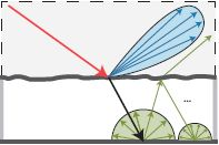
对于以上这种多层次的材质，如果不考虑不咋的层次间的反射和折射的话（通常这一部分对视觉的影响也非常小），直接将Microfacet和漫反射的部分相加就可以得到非常不错的效果。

镜面反射和漫反射的能量的权重需要用电介材质的菲涅尔项进行计算。如果要更加精确的计算不同材质间内部的反射，吸收，以及考虑材质厚度的影响。https://www.cg.tuwien.ac.at/research/publications/2007/weidlich_2007_almfs/weidlich_2007_almfs-paper.pdf

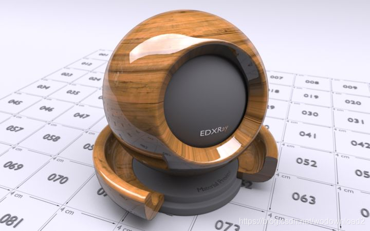
下面是直接将漫反射项和Microfacet项用Fresnel权重相加得到的表面涂有清漆的木材渲染结果。
在这里插入图片描述
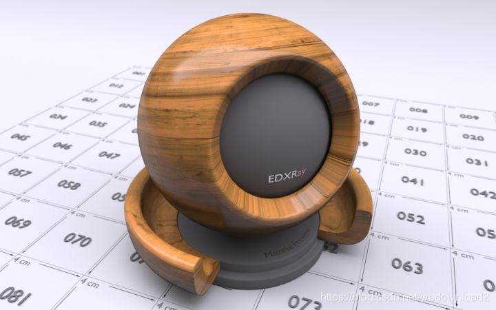
这是表面的清漆不那么光滑的渲染结果。

有了这种模型，就已经可以模拟很大一部分现实中的材质了。但是还有相当一部分的材质，一层漫反射加上一层镜面反射是不足以模拟的，一个非常常见的例子就是车漆。通常车漆是在一层粗糙的金属材质外层涂上一层平滑的透明清漆，所以看起来才有下图的样子，首先有金属的质感，但是同时表面又有非常细致的镜面反射。
在这里插入图片描述
这一类材质的光线传递示意图如下：

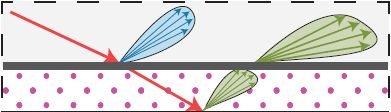
所以对于这种材质来说则需要多次用Fresnel项去叠加两个Microfacet镜面反射。就可以渲染出下图中的材质。

http://www.codinglabs.net/article_physically_based_rendering_cook_torrance.aspx

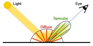
cook-torrance brdf is a function that can be plugged into the rendering equation as fr. with this brdf we model the behaviour of light in two different ways making a distinction between diffuse reflection and specular reflection. the idea is that the material we are simulating reflects a certain amount of light in all directions (Lambert) and another amount in a specular way (like a mirror). because of this the cook-torrance brdf does not completely replace the one we have previously but instead, with this new model, we will able to specify how much radiacne is diffused and how much is reflected in a specular way depending on what material we are trying to simulate. the brdf function fr looks like this:
在这里插入图片描述

在这里插入图片描述

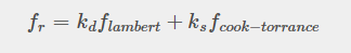
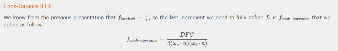
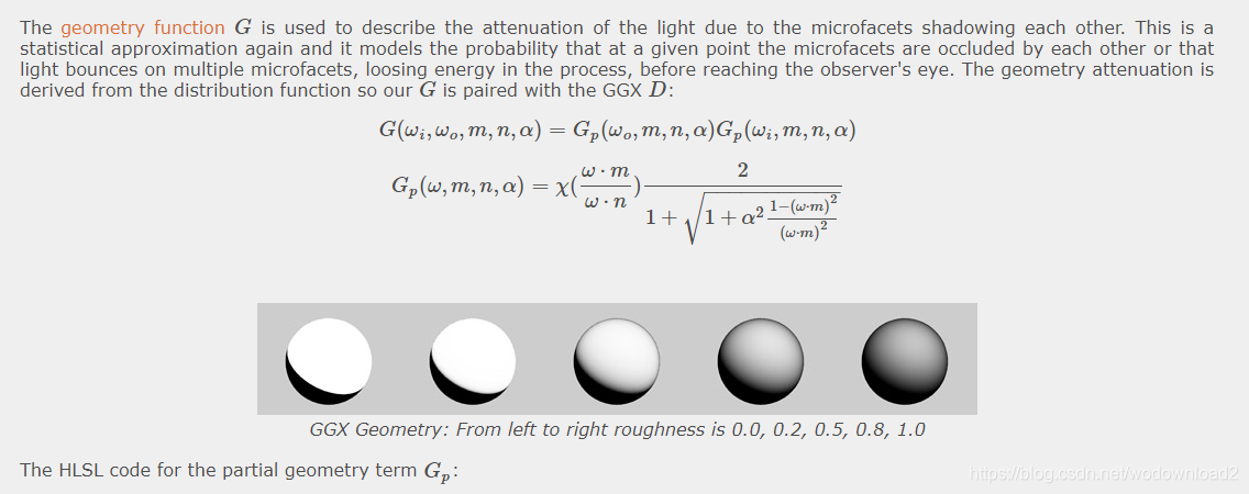
where D is the distribution function , F is the fresnel function and G is the geometry function. these three functions are the backbone of the cook-torrance model and each one tries to model a specific behaviour of the surface’s material we are trying to simulate. the approximation model of the surface that cook and torrance have used falls into the categroy of the microfacet models which revolves 旋转 around the idea that rough surfaces can be modelled as a collection of small microfacets. these microfacets are assumed to be very small perfect reflectors and their behaviour is described by statistical models, and in our case both functoins D and G are based on this idea.

he distribution function D is used to describe the statistical orientation of the micro facets at some given point. For example if 20% of the facets are oriented facing some vector m, feeding m into the distribution function will give us back 0.2. There are several functions in literature to describe this distributions (such as Phong, or Beckmann) but the function that we will use for our distribution will be the GGX [1] which is defined as follow:
在这里插入图片描述
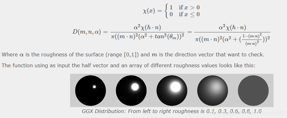
As you can see when the roughness is low (leftmost image) only a few points are oriented towards the half vector, but within those points a great quantity of microfacets are oriented that way and this is represented by the white output. When the roughness is higher more and more points have some percentage of microfacets oriented the same way of the half vector, within those points there are only a handful of microfacets oriented the right way and this is represented by the gray colour. The HLSL code reads as follow:

float chiGGX(float v)
{
    return v > 0 ? 1 : 0;
}

float GGX_Distribution(float3 n, float3 h, float alpha)
{
    float NoH = dot(n,h);
    float alpha2 = alpha * alpha;
    float NoH2 = NoH * NoH;
    float den = NoH2 * alpha2 + (1 - NoH2);
    return (chiGGX(NoH) * alpha2) / ( PI * den * den );
}

在这里插入图片描述

float chiGGX(float v)
{
    return v > 0 ? 1 : 0;
}

float GGX_PartialGeometryTerm(float3 v, float3 n, float3 h, float alpha)
{
    float VoH2 = saturate(dot(v,h));
    float chi = chiGGX( VoH2 / saturate(dot(v,n)) );
    VoH2 = VoH2 * VoH2;
    float tan2 = ( 1 - VoH2 ) / VoH2;
    return (chi * 2) / ( 1 + sqrt( 1 + alpha * alpha * tan2 ) );
}

the fresnel function F is used to simulate the way light interacts with a surface at different angles. the function accepts in input the incoming ray and a few surface’s properties. the actual formular is rather complex and is different for conductive and dielectrics materials, but there is a nice approximated version presented by shlick C. (1994) that can be evaluated very quickly and that we will use for our model (on dielectric materials):
在这里插入图片描述
Where θ is the angle between the viewing direction and the half vector while the parameter η1 and η2 are the indices of refraction (IOR) of the two medias. this formula is an approximation of the full version that describes the interaction of light passing from dielectric to dielectric materials with different index of refraction. if we want t omodel conductor materials we have to use a different formula tought. a good approximation for conductors is given by the following:
在这里插入图片描述
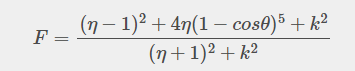
Where θ is the angle between the viewing direction and the half vector, ηη is the index of refraction for the conductor and k is the absorption coefficient of the conductor. The formula assumes the media where the ray is coming from is air or vacuum.

在这里插入图片描述

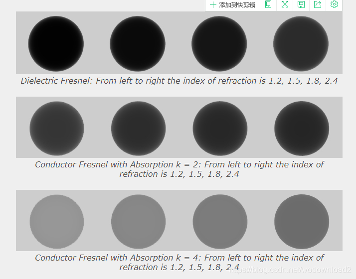
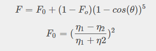
as u can see above the two function give very different resutls and depending of what material we are trying to simulate we would have to pick one formula or the other. we could use the formulas as presented, but the correct trend, used by the top notch engines like unreal, is to approximate even more using a concept introduced in the cook-torrance paper: the idea of reflectance at normal incidence. To keep the math simple the idea is to precalculate the material’s response at normal incidence and then interpolate this value based on the view angle. This is also based on Schlick’s approximation:

float3 Fresnel_Schlick(float cosT, float3 F0)
{
  return F0 + (1-F0) * pow( 1 - cosT, 5);
}

Where F0 is the material’s response at normal incidence. We calculate F0 as follow:

// Calculate colour at normal incidence
float3 F0 = abs ((1.0 - ior) / (1.0 + ior));
F0 = F0 * F0;
F0 = lerp(F0, materialColour.rgb, metallic);