


一、基本概念
参考:Robot Localization AMCL原理以及代码_sinat_37011812的博客-CSDN博客
注释:本部分内容CSDN上多个博主都有介绍,不知道谁是原创。暂且附上上述链接。
先讲几个坐标系的关系吧,在机器人定位中很重要。
base_link 一般指的是机器人自身的坐标系,随着机器人的移动而移动。
odom的原点是机器人刚启动时刻的位置,理论上这个odom坐标系是固定的不会变化的,但是odom是会随着时间发生漂移且存在累积误差,因此odom坐标系实际上会随着时间移动
map是地图的坐标系,当地图建立完成之后,map坐标系就固定下来了,不会随时间发生变化。
一般我们的odom坐标系和map坐标系是重合的,假设机器人启动位置就是地图的原点
一般机器人定位时坐标系的关系是 base_link <-> odom <-> map
这里 base_link <-> odom两个坐标系时间的转换关系一般由里程计odomerty,IMU或者视觉里程计提供。
由于odom会发生漂移和累积误差,因此odom<->map之间会有一段未知的、待估计的转换关系
定位一般用base_link <-> map,但是在AMCL中我们估计odom<->map,由此完成机器人的定位问题
Adaptive Monte Carlo Localization
是一套适用于二维机器人运动的定位算法。其主要的算法原理源于《Probabilistic Robotics》一书8.3中描述的MCL, Augmented_MCL, 和KLD_Sampling_MCL算法的结合与实现。同时书中第5章描述的Motion Model和第6章描述的Sensor Model,用于AMCL中运动的预测和粒子权重的更新。
1,粒子滤波和蒙特卡洛
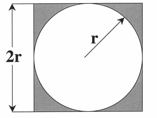
蒙特卡洛:是一种思想或方法。举例:一个矩形里面有个不规则形状,怎么计算不规则形状的面积?不好算。但我们可以近似。拿一堆豆子,均匀的撒在矩形上,然后统计不规则形状里的豆子的个数和剩余地方的豆子个数。矩形面积知道的呀,所以就通过估计得到了不规则形状的面积。拿机器人定位来讲,它处在地图中的任何一个位置都有可能,这种情况我们怎么表达一个位置的置信度呢?我们也使用粒子,哪里的粒子多,就代表机器人在哪里的可能性高。
粒子滤波:粒子数代表某个东西的可能性高低。通过某种评价方法(评价这个东西的可能性),改变粒子的分布情况。比如在机器人定位中,某个粒子A,我觉得这个粒子在这个坐标(比如这个坐标就属于之前说的“这个东西”)的可能性很高,那么我给他打高分。下次重新安排所有的粒子的位置的时候,就在这个位置附近多安排一些。这样多来几轮,粒子就都集中到可能性高的位置去了。
2,重要性采样
就像转盘抽奖一样,原本分数高(我们给它打分)的粒子,它在转盘上对应的面积就大。原本有100个粒子,那下次我就转100次,转到什么就取个对应的粒子。这样多重复几次,仍然是100个粒子,但是分数高的粒子越来越多了,它们代表的东西(比如位姿)几乎是一样的。
3,机器人绑架
举例,机器人突然被抱走,放到了另外一个地方。类似这种情况。
4,自适应蒙特卡洛
解决了机器人绑架问题,它会在发现粒子们的平均分数突然降低了(意味着正确的粒子在某次迭代中被抛弃了)的时候,在全局再重新的撒一些粒子。
解决了粒子数固定的问题,因为有时候当机器人定位差不多得到了的时候,比如这些粒子都集中在一块了,还要维持这么多的粒子没必要,这个时候粒子数可以少一点了。
5,KLD采样
就是为了控制上述粒子数冗余而设计的。比如在栅格地图中,看粒子占了多少栅格。占得多,说明粒子很分散,在每次迭代重采样的时候,允许粒子数量的上限高一些。占得少,说明粒子都已经集中了,那就将上限设低,采样到这个数就行了。
amcl/sensors/odom
case ODOM_MODEL_DIFF:
{
// Implement sample_motion_odometry (Prob Rob p 136)
double delta_rot1, delta_trans, delta_rot2;
double delta_rot1_hat, delta_trans_hat, delta_rot2_hat;
double delta_rot1_noise, delta_rot2_noise;
// Avoid computing a bearing from two poses that are extremely near each
// other (happens on in-place rotation).
if(sqrt(ndata->delta.v[1]*ndata->delta.v[1] +
ndata->delta.v[0]*ndata->delta.v[0]) < 0.01)
delta_rot1 = 0.0;
else
delta_rot1 = angle_diff(atan2(ndata->delta.v[1], ndata->delta.v[0]),
old_pose.v[2]);
delta_trans = sqrt(ndata->delta.v[0]*ndata->delta.v[0] +
ndata->delta.v[1]*ndata->delta.v[1]);
delta_rot2 = angle_diff(ndata->delta.v[2], delta_rot1);
// We want to treat backward and forward motion symmetrically for the
// noise model to be applied below. The standard model seems to assume
// forward motion.
delta_rot1_noise = std::min(fabs(angle_diff(delta_rot1,0.0)),
fabs(angle_diff(delta_rot1,M_PI)));
delta_rot2_noise = std::min(fabs(angle_diff(delta_rot2,0.0)),
fabs(angle_diff(delta_rot2,M_PI)));
for (int i = 0; i < set->sample_count; i++)
{
pf_sample_t* sample = set->samples + i;
// Sample pose differences
delta_rot1_hat = angle_diff(delta_rot1,
pf_ran_gaussian(this->alpha1*delta_rot1_noise*delta_rot1_noise +
this->alpha2*delta_trans*delta_trans));
delta_trans_hat = delta_trans -
pf_ran_gaussian(this->alpha3*delta_trans*delta_trans +
this->alpha4*delta_rot1_noise*delta_rot1_noise +
this->alpha4*delta_rot2_noise*delta_rot2_noise);
delta_rot2_hat = angle_diff(delta_rot2,
pf_ran_gaussian(this->alpha1*delta_rot2_noise*delta_rot2_noise +
this->alpha2*delta_trans*delta_trans));
// Apply sampled update to particle pose
sample->pose.v[0] += delta_trans_hat *
cos(sample->pose.v[2] + delta_rot1_hat);
sample->pose.v[1] += delta_trans_hat *
sin(sample->pose.v[2] + delta_rot1_hat);
sample->pose.v[2] += delta_rot1_hat + delta_rot2_hat;
}
}
amcl/sensors/laser
// Determine the probability for the given pose
double AMCLLaser::BeamModel(AMCLLaserData *data, pf_sample_set_t* set)
{
AMCLLaser *self;
int i, j, step;
double z, pz;
double p;
double map_range;
double obs_range, obs_bearing;
double total_weight;
pf_sample_t *sample;
pf_vector_t pose;
self = (AMCLLaser*) data->sensor;
total_weight = 0.0;
// Compute the sample weights
for (j = 0; j < set->sample_count; j++)
{
sample = set->samples + j;
pose = sample->pose;
// Take account of the laser pose relative to the robot
pose = pf_vector_coord_add(self->laser_pose, pose);
p = 1.0;
step = (data->range_count - 1) / (self->max_beams - 1);
for (i = 0; i < data->range_count; i += step)
{
obs_range = data->ranges[i][0];
obs_bearing = data->ranges[i][1];
// Compute the range according to the map
map_range = map_calc_range(self->map, pose.v[0], pose.v[1],
pose.v[2] + obs_bearing, data->range_max);
pz = 0.0;
// Part 1: good, but noisy, hit
z = obs_range - map_range;
pz += self->z_hit * exp(-(z * z) / (2 * self->sigma_hit * self->sigma_hit));
// Part 2: short reading from unexpected obstacle (e.g., a person)
if(z < 0)
pz += self->z_short * self->lambda_short * exp(-self->lambda_short*obs_range);
// Part 3: Failure to detect obstacle, reported as max-range
if(obs_range == data->range_max)
pz += self->z_max * 1.0;
// Part 4: Random measurements
if(obs_range < data->range_max)
pz += self->z_rand * 1.0/data->range_max;
// TODO: outlier rejection for short readings
assert(pz <= 1.0);
assert(pz >= 0.0);
// p *= pz;
// here we have an ad-hoc weighting scheme for combining beam probs
// works well, though...
p += pz*pz*pz;
}
sample->weight *= p;
total_weight += sample->weight;
}
return(total_weight);
}
double AMCLLaser::LikelihoodFieldModel(AMCLLaserData *data, pf_sample_set_t* set)
{
AMCLLaser *self;
int i, j, step;
double z, pz;
double p;
double obs_range, obs_bearing;
double total_weight;
pf_sample_t *sample;
pf_vector_t pose;
pf_vector_t hit;
self = (AMCLLaser*) data->sensor;
total_weight = 0.0;
// Compute the sample weights
for (j = 0; j < set->sample_count; j++)
{
sample = set->samples + j;
pose = sample->pose;
// Take account of the laser pose relative to the robot
pose = pf_vector_coord_add(self->laser_pose, pose);
p = 1.0;
// Pre-compute a couple of things
double z_hit_denom = 2 * self->sigma_hit * self->sigma_hit;
double z_rand_mult = 1.0/data->range_max;
step = (data->range_count - 1) / (self->max_beams - 1);
// Step size must be at least 1
if(step < 1)
step = 1;
for (i = 0; i < data->range_count; i += step)
{
obs_range = data->ranges[i][0];
obs_bearing = data->ranges[i][1];
// This model ignores max range readings
if(obs_range >= data->range_max)
continue;
// Check for NaN
if(obs_range != obs_range)
continue;
pz = 0.0;
// Compute the endpoint of the beam
hit.v[0] = pose.v[0] + obs_range * cos(pose.v[2] + obs_bearing);
hit.v[1] = pose.v[1] + obs_range * sin(pose.v[2] + obs_bearing);
// Convert to map grid coords.
int mi, mj;
mi = MAP_GXWX(self->map, hit.v[0]);
mj = MAP_GYWY(self->map, hit.v[1]);
// Part 1: Get distance from the hit to closest obstacle.
// Off-map penalized as max distance
if(!MAP_VALID(self->map, mi, mj))
z = self->map->max_occ_dist;
else
z = self->map->cells[MAP_INDEX(self->map,mi,mj)].occ_dist;
// Gaussian model
// NOTE: this should have a normalization of 1/(sqrt(2pi)*sigma)
pz += self->z_hit * exp(-(z * z) / z_hit_denom);
// Part 2: random measurements
pz += self->z_rand * z_rand_mult;
// TODO: outlier rejection for short readings
assert(pz <= 1.0);
assert(pz >= 0.0);
// p *= pz;
// here we have an ad-hoc weighting scheme for combining beam probs
// works well, though...
p += pz*pz*pz;
}
sample->weight *= p;
total_weight += sample->weight;
}
return(total_weight);
}
particle filter
void pf_update_sensor(pf_t *pf, pf_sensor_model_fn_t sensor_fn, void *sensor_data)
{
int i;
pf_sample_set_t *set;
pf_sample_t *sample;
double total;
set = pf->sets + pf->current_set;
// Compute the sample weights
total = (*sensor_fn) (sensor_data, set);
if (total > 0.0)
{
// Normalize weights
double w_avg=0.0;
for (i = 0; i < set->sample_count; i++)
{
sample = set->samples + i;
w_avg += sample->weight;
sample->weight /= total;
}
// Update running averages of likelihood of samples (Prob Rob p258)
w_avg /= set->sample_count;
if(pf->w_slow == 0.0)
pf->w_slow = w_avg;
else
pf->w_slow += pf->alpha_slow * (w_avg - pf->w_slow);
if(pf->w_fast == 0.0)
pf->w_fast = w_avg;
else
pf->w_fast += pf->alpha_fast * (w_avg - pf->w_fast);
//printf("w_avg: %e slow: %e fast: %e\n",
//w_avg, pf->w_slow, pf->w_fast);
}
else
{
// Handle zero total
for (i = 0; i < set->sample_count; i++)
{
sample = set->samples + i;
sample->weight = 1.0 / set->sample_count;
}
}
return;
}
// Resample the distribution
void pf_update_resample(pf_t *pf)
{
int i;
double total;
pf_sample_set_t *set_a, *set_b;
pf_sample_t *sample_a, *sample_b;
//double r,c,U;
//int m;
//double count_inv;
double* c;
double w_diff;
set_a = pf->sets + pf->current_set;
set_b = pf->sets + (pf->current_set + 1) % 2;
// Build up cumulative probability table for resampling.
// TODO: Replace this with a more efficient procedure
// (e.g., http://www.network-theory.co.uk/docs/gslref/GeneralDiscreteDistributions.html)
c = (double*)malloc(sizeof(double)*(set_a->sample_count+1));
c[0] = 0.0;
for(i=0;i<set_a->sample_count;i++)
c[i+1] = c[i]+set_a->samples[i].weight;
// Create the kd tree for adaptive sampling
pf_kdtree_clear(set_b->kdtree);
// Draw samples from set a to create set b.
total = 0;
set_b->sample_count = 0;
w_diff = 1.0 - pf->w_fast / pf->w_slow;
if(w_diff < 0.0)
w_diff = 0.0;
//printf("w_diff: %9.6f\n", w_diff);
// Can't (easily) combine low-variance sampler with KLD adaptive
// sampling, so we'll take the more traditional route.
/*
// Low-variance resampler, taken from Probabilistic Robotics, p110
count_inv = 1.0/set_a->sample_count;
r = drand48() * count_inv;
c = set_a->samples[0].weight;
i = 0;
m = 0;
*/
while(set_b->sample_count < pf->max_samples)
{
sample_b = set_b->samples + set_b->sample_count++;
if(drand48() < w_diff)
sample_b->pose = (pf->random_pose_fn)(pf->random_pose_data);
else
{
// Can't (easily) combine low-variance sampler with KLD adaptive
// sampling, so we'll take the more traditional route.
/*
// Low-variance resampler, taken from Probabilistic Robotics, p110
U = r + m * count_inv;
while(U>c)
{
i++;
// Handle wrap-around by resetting counters and picking a new random
// number
if(i >= set_a->sample_count)
{
r = drand48() * count_inv;
c = set_a->samples[0].weight;
i = 0;
m = 0;
U = r + m * count_inv;
continue;
}
c += set_a->samples[i].weight;
}
m++;
*/
// Naive discrete event sampler
double r;
r = drand48();
for(i=0;i<set_a->sample_count;i++)
{
if((c[i] <= r) && (r < c[i+1]))
break;
}
assert(i<set_a->sample_count);
sample_a = set_a->samples + i;
assert(sample_a->weight > 0);
// Add sample to list
sample_b->pose = sample_a->pose;
}
sample_b->weight = 1.0;
total += sample_b->weight;
// Add sample to histogram
pf_kdtree_insert(set_b->kdtree, sample_b->pose, sample_b->weight);
// See if we have enough samples yet
if (set_b->sample_count > pf_resample_limit(pf, set_b->kdtree->leaf_count))
break;
}
// Reset averages, to avoid spiraling off into complete randomness.
if(w_diff > 0.0)
pf->w_slow = pf->w_fast = 0.0;
//fprintf(stderr, "\n\n");
// Normalize weights
for (i = 0; i < set_b->sample_count; i++)
{
sample_b = set_b->samples + i;
sample_b->weight /= total;
}
// Re-compute cluster statistics
pf_cluster_stats(pf, set_b);
// Use the newly created sample set
pf->current_set = (pf->current_set + 1) % 2;
pf_update_converged(pf);
free(c);
return;
}
// Compute the required number of samples, given that there are k bins
// with samples in them. This is taken directly from Fox et al.
int pf_resample_limit(pf_t *pf, int k)
{
double a, b, c, x;
int n;
if (k <= 1)
return pf->max_samples;
a = 1;
b = 2 / (9 * ((double) k - 1));
c = sqrt(2 / (9 * ((double) k - 1))) * pf->pop_z;
x = a - b + c;
n = (int) ceil((k - 1) / (2 * pf->pop_err) * x * x * x);
if (n < pf->min_samples)
return pf->min_samples;
if (n > pf->max_samples)
return pf->max_samples;
return n;
}
Reference
http://wiki.ros.org/amcl
https://github.com/ros-planning/navigation/tree/melodic-devel/amcl
https://robomaster.github.io/RoboRTS-Tutorial/#/sdk_docs/roborts_localization?id=amcl算法
https://github.com/RoboMaster/RoboRTS/tree/ros/roborts_localization/amcl
https://cse.sc.edu/~terejanu/files/tutorialMC.pdf
https://blog.csdn.net/hmbxsy/article/details/80509876
https://blog.csdn.net/wyang9x/article/details/84034333
https://blog.csdn.net/u013834525/article/details/80166552
https://blog.csdn.net/xyz599/article/details/52942485
https://blog.csdn.net/crazyquhezheng/article/details/49154805
https://blog.csdn.net/ethan_guo/article/details/81809054
注释:蒙特卡洛应用举例:蒙特卡罗方法入门 - 阮一峰的网络日志
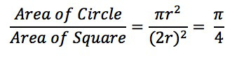
用蒙特卡罗方法计算圆周率π。正方形内部有一个相切的圆,它们的面积之比是π/4。
现在,在这个正方形内部,随机产生10000个点(即10000个坐标对 (x, y)),计算它们与中心点的距离,从而判断是否落在圆的内部。
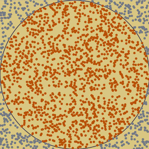
如果这些点均匀分布,那么圆内的点应该占到所有点的 π/4,因此将这个比值乘以4,就是π的值。通过R语言脚本随机模拟30000个点,π的估算值与真实值相差0.07%。
二、ROS Navigation之amcl源码解析(完全详解)
参考1:ROS Navigation之amcl源码解析(完全详解)_sakura123.的博客-CSDN博客
参考2:ROS amcl定位参数解析 配置_Rosabor的博客-CSDN博客_amcl参数
X. ROS官方给了一些解释:amcl - ROS Wiki
Algorithms
Many of the algorithms and their parameters are well-described in the book Probabilistic Robotics, by Thrun, Burgard, and Fox. The user is advised to check there for more detail. In particular, we use the following algorithms from that book: sample_motion_model_odometry, beam_range_finder_model, likelihood_field_range_finder_model, Augmented_MCL, and KLD_Sampling_MCL.
As currently implemented, this node works only with laser scans and laser maps. It could be extended to work with other sensor data.
说明ROS官方的amcl不是一个特定的定位算法,而是集成了一类模型和算法的策略集合。
三、网友分析amcl源代码系列


 3491
3491

 被折叠的 条评论
为什么被折叠?
被折叠的 条评论
为什么被折叠?
 到【灌水乐园】发言


