使用Python动画粒子的薛定谔波函数（ψ）（完整代码）

左图：来源，右图：作者生成

 

一、说明

        物质的双重性质是物理学家中一个著名的概念。原子尺度的物质在某些情况下表现为粒子，而在某些情况下，它们的行为类似于波。为了解释这一点，我们引入了波函数ψ（x，t），它描述的不是粒子的实际位置，而是在给定点找到粒子的概率。波函数ψ（x，t）或概率场，满足一个也许是最重要的偏微分方程，至少对物理学家来说是这样，是薛定谔方程。

薛定谔方程， 

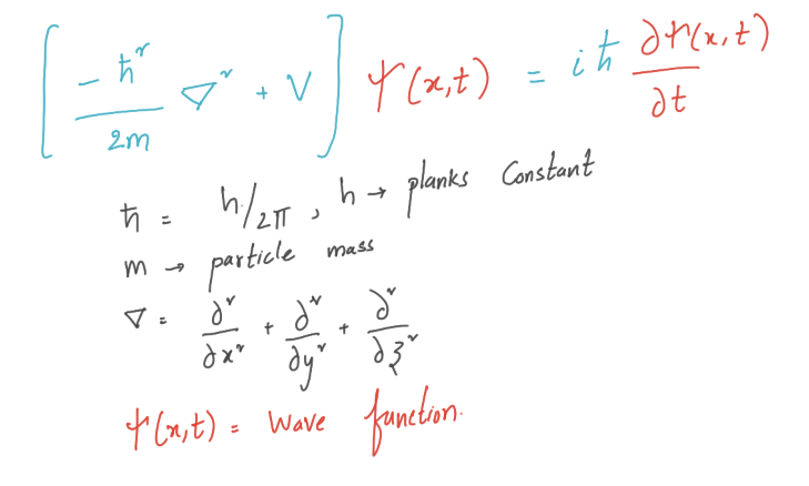
二、一维薛定谔方程

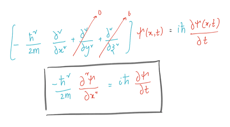
        我们将在一个维度上研究薛定谔方程。求解二维或三维波函数的方法与求解一维波函数的方法基本相同。但为了可视化和时间关系，我们将坚持一个维度。让我们推导出一维情况的薛定谔方程。

一维薛定谔方程 

三、使用曲柄-尼科尔森方法求解盒子中的粒子

框，由作者生成

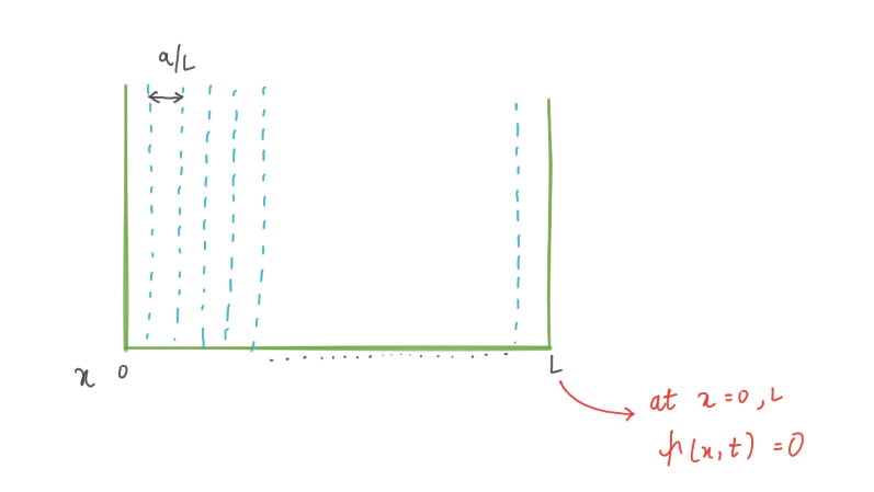
        我们将求解一个粒子的波动方程，该粒子位于一个具有不可穿透墙壁的盒子中。这个想法是在有限大小的空间中求解方程。但为什么要在坚不可摧的墙壁上呢？这个条件迫使波函数在壁上为零，我们将把波函数放在 x = 0 和 x = L 处。我们将用有限差值替换薛定谔方程中的二阶导数，并应用欧拉方法。

将欧拉方法应用于一维薛定谔方程

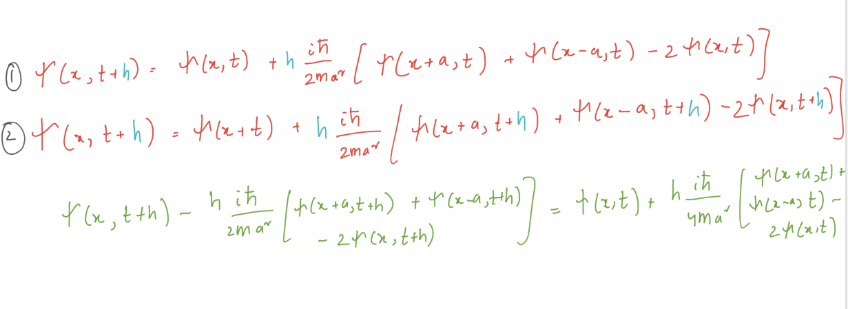
        上述推导使我们能够递归地求解薛定谔方程。 x = 0 和 x = L 处的边界条件对于所有 t 波函数 ψ(x,t) = 0 。在这些点之间，我们在 a、2a、3a 等处有网格点。让我们将这些内部点的值 ψ(x,t) 排列成一个向量。

使用三对角线方法求解曲柄-尼科尔森方程，由作者生成

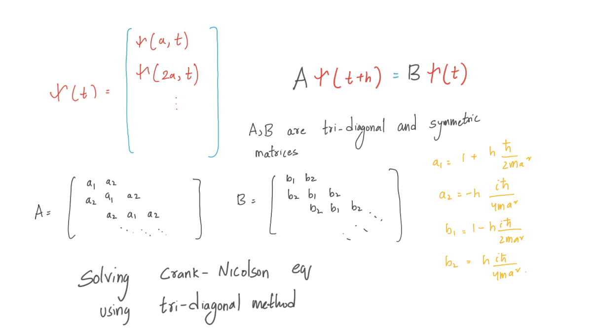
        现在事情很简单了，我们有一个传播函数：
        A ψ（t+h） = B ψ（t），其中矩阵 A 和 B既对称又是三对角线。我们必须在时间步长 t= 0 ， ψ（0） 初始化波函数。使用传播函数，我们可以近似ψ（h），然后使用ψ（h）我们可以近似ψ（2h）等等。在时间t = 0时，粒子的波函数ψ（0）具有这种形式。

波函数 ψ（0）

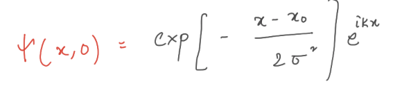
        ψ（0） 的这个表达式没有归一化，实际上应该有一个整体乘法系数，以确保粒子的概率密度积分为单位。

四、框中粒子的波函数动画

        我们将尝试使用Crank-Nicolson方法在具有不可穿透墙壁的盒子中对粒子进行动画处理。我们需要计算网格上所有时间步长的向量 ψ（x， t），给定初始波函数 ψ（0） 并使用切片长度 = L/N 的空间切片 （N = 1000）。

 

盒子中粒子的波函数动画 

五、完整实验代码 

import numpy  as np
from pylab import *
from matplotlib import pyplot as plt
from matplotlib import animation
#matplotlib.use('GTK3Agg') 

# from matplotlib import interactive
# interactive(True)

########################################Variables######################################################################################################
N_Slices = 1000            #Number of slices in the box 
Time_step = 1e-18          #Time step for each iteration 
Mass = 9.109e-31           #mass of electron 
plank = 1.0546e-36         #Planks constant 
L_Box = 1e-9           #Length of the box
Grid = L_Box/N_Slices                             #Lenght of each slice 

#####################################Si(0) using the given equation ###############################################################################


Si_0 = np.zeros(N_Slices+1,complex)                        #Initiating Si funtion at time step = 0 
x = np.linspace(0,L_Box,N_Slices+1)                            
def G_Equation(x):
    x_0 = L_Box/2
    Sig = 1e-10
    k = 5e10
    result  = exp(-(x-x_0)**2/2/Sig**2)*exp(1j*k*x)       #Given Equation at t = 0
    return result
Si_0[:] = G_Equation(x)                                     #Si funtion at time step = 0           


#######################################V = Bxsi(0)################################################################################
a_1 = 1 + Time_step*plank*1j/(2*Mass*(Grid**2))   #Diagonal of A Tridiagonal matrix
a_2 = -Time_step*plank*1j/(4*Mass*Grid**2)        #Up and Down to A Tridiagonal matrix
b_1 =  1 - Time_step*plank*1j/(2*Mass*(Grid**2))  #Diagonal of B Tridiagonal matrix
b_2 =  Time_step*plank*1j/(4*Mass*Grid**2)        #Up and Down to B Tridiagonal matrix



BxSi_0 = []                                                      #V = BxSi and si funtion at x = 0
for i in range(1000):
    if i == 0:
        BxSi_0.append(b_1*Si_0[0] + b_2*(Si_0[1]))                   #V can be maipulated by the equation in Text book          
    else:                                                     
        BxSi_0.append(b_1*Si_0[i] + b_2*(Si_0[i+1] + Si_0[i-1]))
BxSi_0 = np.array(BxSi_0)

#####################################Tri Diagonal matrix algorithm#####################################################################################

def TDMAsolver(a, b, c, d):                                   #Instead of solving using Numpy.linalg, it is prefered to Use 
    nf = len(d)                                               #Tri Diagonal Matrix algorithm 
    ac, bc, cc, dc = map(np.array, (a, b, c, d))              # a,b,c's are up,dia,down element in tridiagonl matrix A
    for it in range(1, nf):                                  #AX = d
        mc = ac[it-1]/bc[it-1]
        bc[it] = bc[it] - mc*cc[it-1] 
        dc[it] = dc[it] - mc*dc[it-1]
        	    
    xc = bc
    xc[-1] = dc[-1]/bc[-1]

    for il in range(nf-2, -1, -1):
        xc[il] = (dc[il]-cc[il]*xc[il+1])/bc[il]
    return xc


global a                    #A matrix is fixed through out the problem, so it is good to globalize the variables 
global b
global c
b = N_Slices*[a_1]          #In A matrix, Both  Up,Down elements are a_2 and diag matrix is a_1
a = (N_Slices-1)*[a_2]
c = (N_Slices-1)*[a_2]
####################################Si 1st funtion solver####################################################################################

global Si_1                                 #First si_funtion usinf Axsi(0+h) = BxSi(0)
Si_1 = TDMAsolver(a, b, c, BxSi_0)          #This can be solved by TDM(A,BxSi(0))


###################################A funtion which caliculates si at each step#####################################################################################
global Si_sd                            #AxSi_stepup = BxSi_stepdown
Si_sd = {}                              #At first Buckting Si_stepdown in to directry which we can using for finding Si_stepup 
def sifuntion(i):                       #In next iteration, Last iteration Si_stepup will be this iteration's Si_stepdown
    if i == 0:
        Si_sd[0] = Si_1
        return Si_1
    else:
        Si_stepdown = Si_sd[i-1]
        V = np.zeros(N_Slices,complex)
        V[0] = b_1*Si_stepdown[0] + b_2*(Si_stepdown[1])
        V[1:N_Slices-1] = b_1*Si_stepdown[1:N_Slices-1] + b_2*(Si_stepdown[2:N_Slices] + Si_stepdown[0:N_Slices-2])
        V[N_Slices-1] = b_1*Si_stepdown[N_Slices-1]+ b_2*(Si_stepdown[N_Slices-2])
        Si_stepup = TDMAsolver(a, b, c, V)
        Si_sd[i] = Si_stepup 
        x = Si_stepup.real
        return x
####################################Animating#######################################################################################
    

fig = plt.figure()
ax = plt.axes(xlim=(0, 1000), ylim=(-1.5, 1.5))
line, = ax.plot([], [], lw=5)
ax.legend(prop=dict(size=20))
ax.set_facecolor('black')
ax.patch.set_alpha(0.8)
ax.set_xlabel('$x$',fontsize = 15,color = 'blue')
ax.set_ylabel(r'$|\psi(x)|$',fontsize = 15,color = 'blue')
ax.grid(color = 'blue')
ax.set_title(r'$|\psi(x)|$ vs $x$', color='blue',fontsize = 15 )
line, = ax.step([], [])

def init():
    line.set_data([], [])
    return line,


def animate(i):
    x = np.linspace(0, 1000, num=1000)
    y = sifuntion(i)
    line.set_data(x, y)
    line.set_color('red')
    return line,

anim = animation.FuncAnimation(fig, animate, init_func=init,
                               frames=10**5, interval=1, blit=True)#5*10**5

plt.vlines(1, -5, 5, linestyles = 'solid', color= 'green',lw=5)
plt.vlines(999, -5, 5, linestyles = 'solid', color= 'green',lw=5)
plt.text(1,1,'Boundary',rotation=90,color= 'green' )
plt.text(975,1,'Boundary',rotation=90,color= 'green' )
plt.figure(figsize=(10,10))
plt.show()   

# Writer = animation.writers['ffmpeg']
# writer = Writer()
# anim.save('im.mp4', writer=writer)