跟着Cell学单细胞转录组分析(九):Monocle2拟时分析演示（上）

最新推荐文章于 2025-03-12 08:56:57 发布

TS的美梦

最新推荐文章于 2025-03-12 08:56:57 发布

阅读量1.1w

点赞数 7

文章标签： r语言数据挖掘数据分析

本文链接：https://blog.csdn.net/qq_42090739/article/details/123497424

版权

该教程详细介绍了如何使用R语言的Monocle包进行单细胞转录组数据的拟时分析。首先，通过安装和加载必要的R包，构建拟时分析所需的CDS对象，接着进行数据预处理，包括基因筛选和降维。然后，进行了差异基因测试并挑选显著性基因，最后通过降维和排序推断细胞分化轨迹，并可视化了基因表达随时间变化的图谱。整个过程为单细胞转录组的拟时分析提供了清晰的步骤和可视化结果。

摘要生成于 C知道，由 DeepSeek-R1 满血版支持，前往体验 >

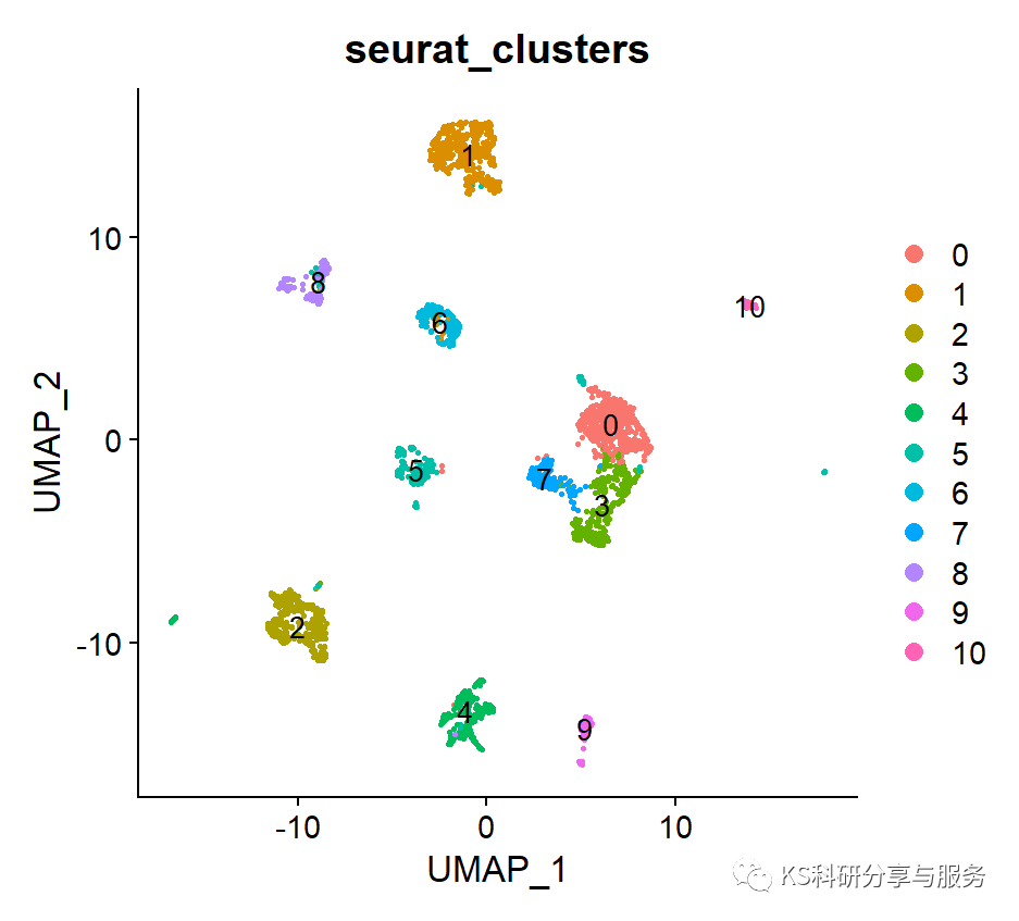
拟时分析是单细胞转录组高级分析内容，也是比较有价值的分析，拟时分析基本使用的都是monocle包，用的最多的是monocle2，我们以之前immun细胞中的0，3，7群Macrophage为例，数据没有意义，仅演示拟时分析。更多详细的拟时分析原理，内容解析可以参考官网：http://cole-trapnell-lab.github.io/monocle-release/docs/。

加载R包，构建拟时分析文件。


if (!requireNamespace("BiocManager", quietly = TRUE))
  install.packages("BiocManager")
BiocManager::install("monocle")
library(monocle)#monocle构建CDS需要3个矩阵：expr.matrix、pd、featuredata
sample_ann <-  Macro@meta.data 
#构建featuredata，一般featuredata需要两个col，一个是gene_id,一个是gene_short_name,row对应counts的rownames
gene_ann <- data.frame(gene_short_name = rownames(Macro@assays$RNA),
                       row.names =  rownames(Macro@assays$RNA))
#head(gene_ann)
pd <- new("AnnotatedDataFrame",data=sample_ann)
fd <- new("AnnotatedDataFrame",data=gene_ann)
#构建matrix
ct=as.data.frame(Macro@assays$RNA@counts)#单细胞counts矩阵

有了matrix，pd，fd，就可以构建monocle对象，进行预处理。

#构建monocle对象
sc_cds <- newCellDataSet(
  as.matrix(ct), 
  phenoData = pd,
  featureData =fd,
  expressionFamily = negbinomial.size(),
  lowerDetectionLimit=1)
sc_cds <- detectGenes(sc_cds, min_expr = 1) 
sc_cds <- sc_cds[fData(sc_cds)$num_cells_expressed > 10, ]
cds <- sc_cds
cds <- estimateSizeFactors(cds)
cds <- estimateDispersions(cds)

基因筛选。


disp_table <- dispersionTable(cds)
unsup_clustering_genes <- subset(disp_table, mean_expression >= 0.1)
cds <- setOrderingFilter(cds, unsup_clustering_genes$gene_id)
plot_ordering_genes(cds) 
plot_pc_variance_explained(cds, return_all = F)

数据降维。


cds <- reduceDimension(cds, max_components = 2, num_dim = 20,
                       reduction_method = 'tSNE', verbose = T)
cds <- clusterCells(cds, num_clusters = 5) 
plot_cell_clusters(cds, 1, 2 )
table(pData(cds)$Cluster) 
colnames(pData(cds))

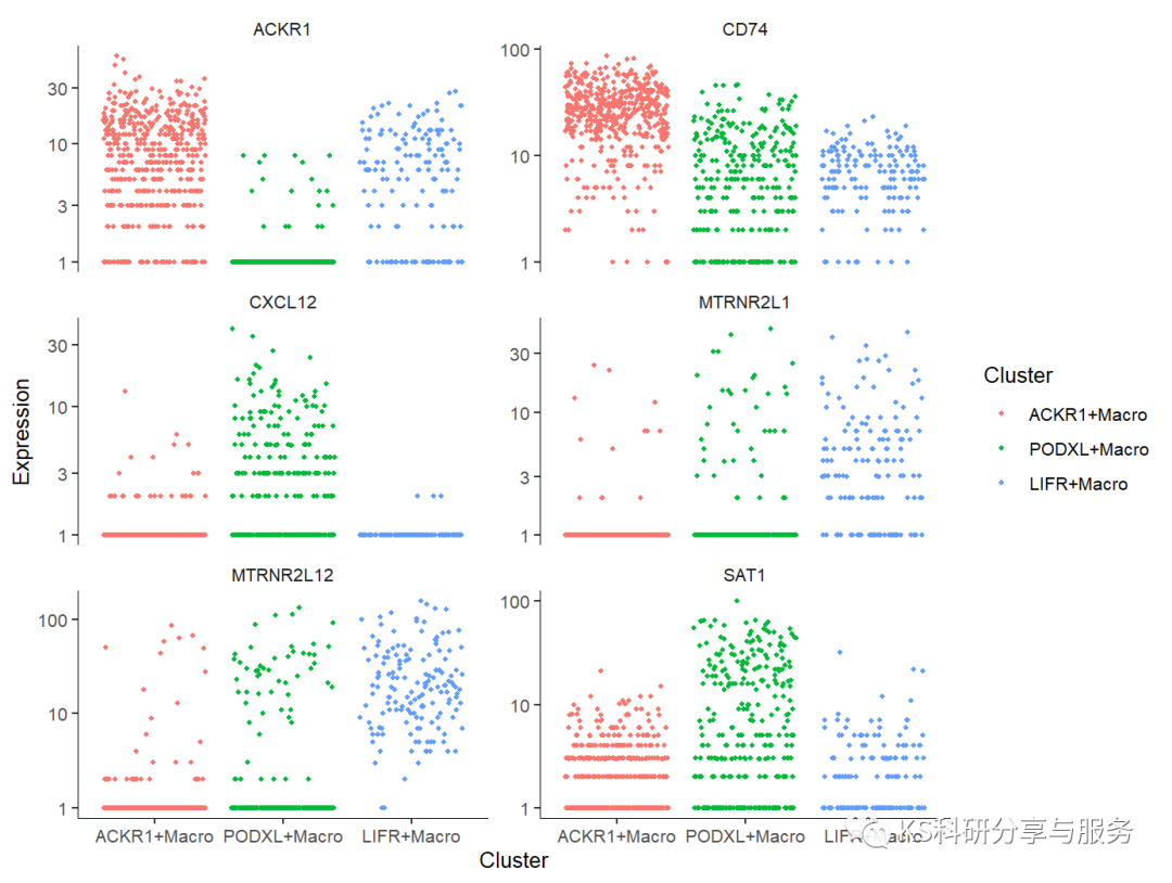
将拟时与seurat分群对应，并挑选显著性基因可视化。

table(pData(cds)$Cluster)
table(pData(cds)$Cluster,pData(cds)$celltype)
pData(cds)$Cluster=pData(cds)$celltype
diff_test_res <- differentialGeneTest(cds, fullModelFormulaStr = "~Cluster")
sig_genes <- subset(diff_test_res, qval < 0.1)
sig_genes=sig_genes[order(sig_genes$pval),]
head(sig_genes[,c("gene_short_name", "pval", "qval")] ) 
cg=as.character(head(sig_genes$gene_short_name)) 
#  挑选差异最显著的基因可视化
plot_genes_jitter(cds[cg,],
                  grouping = "Cluster",
                  color_by = "Cluster",
                  nrow= 3,
                  ncol = NULL )
cg2=as.character(tail(sig_genes$gene_short_name)) 
plot_genes_jitter(cds[cg2,],
                  grouping = "Cluster",
                  color_by = "Cluster",
                  nrow= 3,
                  ncol = NULL )

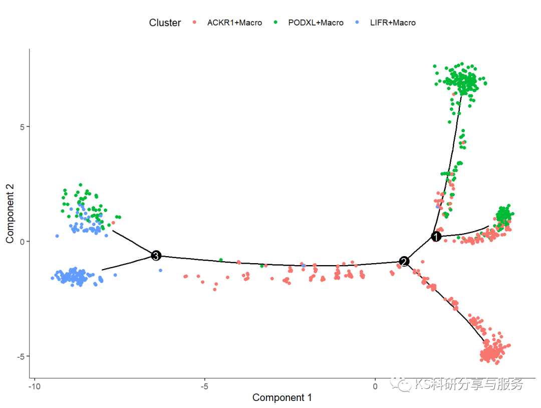
前面差异基因筛选后，开始拟时推测。


# 第一步: 挑选合适的基因
ordering_genes <- row.names (subset(diff_test_res, qval < 0.01))
ordering_genes
cds <- setOrderingFilter(cds, ordering_genes)
plot_ordering_genes(cds)
#第二步降维
cds <- reduceDimension(cds, max_components = 2,
                       method = 'DDRTree')
                       
# 第三步: 对细胞进行排序
cds <- orderCells(cds)
#可视化细胞分化轨迹
plot_cell_trajectory(cds, color_by = "Cluster")

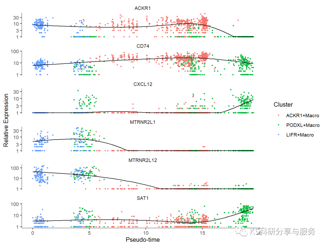
可视化基因时序图。

plot_genes_in_pseudotime(cds[cg,],
                         color_by = "Cluster")

保存拟时cds文件，这将是后期可视化的基础。好了，下节我们将做一下拟时的一些可视化操作，为你的分析添加色彩。