A Quick Introduction to Monte Carlo Methods

https://www.scratchapixel.com/lessons/mathematics-physics-for-computer-graphics/monte-carlo-methods-mathematical-foundations/quick-introduction-to-monte-carlo-methods

Originally we didn’t want the lesson to be so long and to contain so much information about probability and statistics, but the reality is, if you want to understand Monte Carlo methods, you need to cover a lot ground in probability and statistics theory.

In this chapter, we will try to give a sense of what these Monte Carlo methods are, how they work, why, and what they are used for. This quick introduction, is for readers who do not have the time or the desire to get any further. But you may need to read all the remaining chapters if you are serious about learning what these methods are.

This lesson is more an introduction to the mathematical tools upon which the Monte Carlo methods are built. The methods themselves are explained in the next lesson (Monte Carlo Methods in Practice).

A Foreword 前言 about Monte Carlo
Like many other terms which you can frequently spot in CG literature, Monte Carlo appears to many non initiated as a magic word. And to the contrary of some mathematical tools used in computer graphics such a spherical harmonics, which to some degrees are complex (at least compared to Monte Carlo approximation) the principle of the Monte Carlo method is on its own relatively simple (not to say easy). Which is great because this method is extremely handy to solve a wide range of complex problems. Monte Carlo integration or approximation (the two terms can be used however integration is generally better) is probably an old method (the first documented reference to the method can be found in some publications by mathematician Comte de Buffon in the early 18th century) but was only given its current catchy name sometime in the mid 1940s. Monte Carlo is the name of a district in the principality of Monaco famous for its casinos. As we will explain in this lesson, the Monte Carlo method has a lot to do with the field of statistics which on its own is very useful to appreciate your chances to win or lose at a game of chance, such as roulette, anything that involves throwing dice, drawing cards, etc., which can all be seen as random processes. The name is thus quite appropriate as it captures the flavour of what the method does. The method itself, which some famous mathematicians helped to develop and formalize (Fermi, Ulam, von Neumann, Metropolis and others) was critical in the research carried on in developing the atomic bomb (it was used to study the probabilistic behaviour of neutron transport in fissile materials) and its popularity in modern science has a lot to do with computers (von Neumann himself built some of the first computers). Without the use of a computer, Monte Carlo integration is tedious as it requires tons of calculations, which obviously computers are very good at. Now that we have reviewed some history and gave some information about the origin of the method’s name, let’s explain what Monte Carlo is. Unfortunately though as briefly mentioned before, the mathematical meaning of the Monte Carlo method is based on many important concepts from statistics and probability theory. We will first have to review these concepts (and introduce them to you) before looking at the Monte Carlo method itself.

A Quick Introduction to Monte Carlo Methods

What is Monte Carlo? The concept behind MC methods is both simple and robust. However as we will see very soon, it requires potentially massive amount of computation, which is the reason its rise in popularity coincides with the advent of computing technology. Many things in life are too hard to evaluate exactly especially when it involves very large numbers. For example, while not impossible, it could take a very long time to count the number of Jelly beans that a 1 Kg jar may contain. You might count them by hand, one by one, but this might take a very long time (as well as not being the most gratifying job ever). Calculating the average height of the adult population of a country, would require to measure the height of each person making up that population, summing up the numbers and dividing them by total number of people measured. Again, a task that might take a very long time. What we can do instead is take a sample of that population and compute its average height. It is unlikely to give you the exact average height of the entire population, however this technique gives a result which is generally a good approximation of what that number is. We traded off accuracy for speed. Polls also known as statistics are based on this principle which we are all intuitively familiar with. Funnily enough the approximation and the exact average of the entire population might some times be exactly the same. This is only due to chance. In most cases, the numbers will be different.

One question we might want to ask though, is how different? In fact, as the size of the sample increases, this approximation converges to the exact number. In other words, the error between the approximation and the actual result, is getting smaller as the sample size increases. Intuitively, this idea is easy to grasp 领会, however we will see in the next chapter, that it should be (from a mathematical point of view) formulated or interpreted differently. Note that to be fair, elements making the sample need to be chosen randomly with equal probability.

note that the height of a person is a random number. it can be anything really which is the nature of random things. thus, when u sample a population, by randomly picking up elements of that population and measuring their height to approximate the average height, each measure is a random number (since each person from your sample is likely to have a different height). interestingly enough, a sum of random numbers, is another random number. if u can not predict what the number making up the sum are, how can u predict the result of their sum? so, the result of the sum is a random number, and the numbers making up the sum are random numbers.
for a mathematician, the height of a population would be called a random variable, because height among people making up this population varies randomly. we generally denote random variables with upper case letters. the latter X is commonly used.

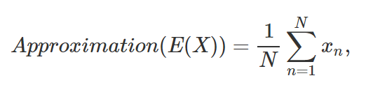
in statistics, the elements making up that population, which as suggested before are random, are denoted with a lower capital letter, generally x as well. for example if we write x2, this would denote the height (which is random) of the second person in the population. all these x’s can also be seen as the possible outcomes of the random variable X. if we call X this random variable (the population height), we can express the concept of approximating the average adult population height from a sample with the following pseudo-mathematical formula:

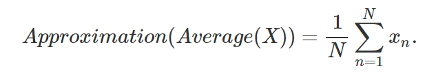
which u can read as, the approximation of the average value of the random variable X, (the height of the adult population of a given country), is equal to the sum (the Σ sign) of the height of N adults randomly chosen from that population (the samples), divided by the number N (the sample size). this in essence, is what we call a monte carlo approximation. it consists of approximating some property of a very large number of things, by avergaing the value of that property for N of these things chosen randomly among all the others. u can also say that Monte Carlo approximation, is in fact a method for approximating things using samples. what we will learn in the next chapters, is that the things which need approximating are called in mathematics expectations (more on this soon). as mentioned before the height of the adult population of a given country can be seen as a random variable X. however note that its average value (which u get by averaging all the height for example of each person making up the population, where each one of these numbers is also a random number) is unique (to avoid the confusion with the sample size which is usually denoted with the letter N, we will use M to denote the size of the entire population):

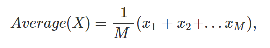
where the x1,x2,…xM corresponds to the height of each person making up the entire population as suggested before (if we were to take an example). In statistics, the average of the random variable X is called an expectation and is written E(X).

to summarize, Monte Carlo approximation (which is one of the MC methods) is a technique to approximate the expection of random variables, using samples. it can be defined mathematically with the following formula:

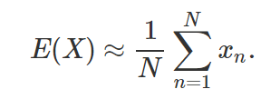
The mathematical sign ≈means that the formula on the right inside of this sign only gives an “approximation” of what the random variable X expectation E(X) actually is. Note that in a way, it’s nothing else than an average of random values (the xns).

if u are just interested in understanding what is hiding behind this mysterious term Monte Carlo, then this all u may want to know about it. however for this quick introduction to be complete, let us explain why this method is useful. it happens as suggested before that computing E(X) is sometimes intractable 棘手的. this means that u can not compute E(X) exactly at least not in an efficient way. This is particularly true when very large “populations” are concerned in the computation of E(X) such as with the case of computing the average height of the adult population of a country. MC approximation offers in this case a very simple and quick way to at least approximate this expectation. It won’t give you the exact value, but it might be close enough at a fraction of the cost of what it might take to compute E(X) exactly, if or possible at all.

Monte Carlo, Biased and Unbiased Ray Tracing

to conclude this quick introduction, we realize that many of u have heard the term monte carlo ray tracing as well as the term of biased and unbiased ray tracing and probably looked at this page, hoping to find an explanation to what these terms mean. let us quickly do it, even though we do recommend that u read the rest of this lesson as well as the following ones, to really get in-depth answers to these questions.

imagine u want to take a picture with a digital camera. if u divide the surface of your images into a regular grid (our pixels), note that each pixel can actually be seen as small but nonetheless continuous surfaces on which light reflected by objects in the scene falls onto. this light will eventually get converted to a single color (and we will talk about this process in a moment) however if u look through any of these pixels, u might notice that it actually sees more than one objects, or that the color of the surface of the object that it sees, varies across the pixel’s area. we have illustrated this idea in firgure 1.

Figure 1: each pixel of an image is actually a small surface. The color of the surface of the object that it sees varies across its area.
what we want to do, ideally, is to compute the amount of light reflected from this surface across the pixel area. while we can write this idea mathematically, there is actually no solution to this equation as such:

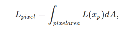
where L here, stands for radiance. u can read this equation as “the actually amount arriving on a pixel (the L term on the left side of the equation which is also the color that will eventually be saved for that pixel) can be computed as the integral of the incoming radiance (light striking the pixel) over the pixel area”. as we just said, there is no analytical solution to this problem thus we need to use a numerical approximation instead.

again the principle here is very simple. it consists of approximating the result of this integral, by sampling the surface of the pixel at several locations across the pixle area. in other words, as with the case of monte carlo approximation, 使用蒙特卡洛, we will use “random sampling” to evaluate this integral (and get an approximation for it). all we need, is to select a few random sample locations across the pixel area and average their color. now is how do we find the color of these samples? using ray tracing of course! rays will start at the eye position as usual but will pass through each randomly placed sample laid out across the area of the pixel (figure 2).

Figure 2: the pixel radiance can be approximated using the average of several randomly selected samples across the surface of that pixel (the black dots). The color of these samples can be found using ray tracing.

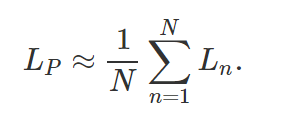
the color of samples will be the color of the rays at their intersection point with the objects from the scene. mathematically, we can write:

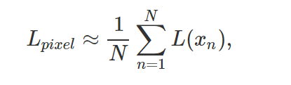
where L(xn) denotes the sample color. as usual, this is only an approximation (hence the ≈ sign). this method is called a monte carlo integration (even though similar to the monte carlo approximation method, it is used in this case to find an approximation to an integral). readers intrested in a formal definition of the monte carlo integration method are referred to the next lesson. this is just an informal and quick introduction to the concept.

if u do not yet understand the problem well, let us just imagine that what we see through a pixel is 16x16 grid of colors (as in depicted in figure 3).

Figure 3: using Monte Carlo to approximate the color of a surface (using 8 samples in this example).

the problem might seems simpler because we only have 256 distinctive colors so in fact, finding out the color of the pixel is feasible in this case: we just need to sum up all these colors and divide the result by 256. but if the grid was inifinitely large, this solution would not work. if we want to find an approximation to this problem, all we need to do is sample say the image in 8 different locations (8 is just an example here. it represents the sample size N and its value can be anything u like), read the color of the grid at these locations, sum up these 8 colors and divide the result by 8. u can see this idea illustrated in figure 3.

as u can see from figure 3, the resulting approximation is close to the average color but a difference is visible. this is the pitfall of monte carlo methods, they just give us approximations. another pitfall of the method is that u will get a different result each time u compute a new approximation. this is due to the random nature of the method (the location of the 8 samples change each time we compute an approximation). for example, the following image shows the result of a series of 16 approximations of the same grid of color using 8 samples.

the good news though, is that u can reduce this error by increasing the number of samples. the bad news, is that no minimize the error by 2, u need twice as many samples. this is the reason why monte carlo methods have the reputation to be slow. a more exactly way of saying this is to say that their rate of convergence (how quickly they converge to the right result as the number of samples increases) is pretty low. this will be studied in detail in this lesson and the following on. the following series of images, show another run of 16 approximations with respectively 8, 16, 32, 64, 128 and 256 samples respectively.

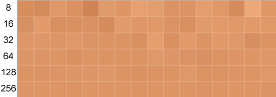
and as expected the difference between each consecutive approximation 连续估计 is reduced as the number of samples increases. this difference in rendering is what u know as noise in your renders (assuming u are using a ray tracer). it is caused by the difference between what the actual solution should be and your approximation. technically the correct name is variance (and probability and statistics have very much to do with the study of variance). u usually get more noise for lower number of samples, 样本越少，噪声越大 or to say it differently by increasing the number of samples, u can reduce the noise (or the variance). 噪声的术语就是方差 however note that the amount of variation u get from one approximation to another (assuming the same number of samples is used) also depends on how much variation there is between the colors from the grid. in the following example, we can see that there is far more color and brightness variation between the colors of the grid than in the previous example. while differences between successive approximations were barely visible in the previous case with 256 samples, with this grid and the same number of samples, differences are more clearly visible.

when does this happen? when u see through a pixel many objects, or see just one or few objects with intricate 复杂的 surface details. generally though, u want to avoid situation where the visual complexity of what u see through a pixel is very large, because the more details the more samples u need to reduce the noise. this idea also relates to the concept of aliasing and the concept of importance sampling. 抗锯齿和重要性采样 here is the code we used to generate these results:看到代码就兴奋

#include <fstream> 
#include <cstdlib> 
#include <cstdio> 
 
int main(int argc, char **argv) 
{ 
        std::ifstream ifs; 
        ifs.open("./tex.pbm"); 
        std::string header; 
        uint32_t w, h, l; 
        ifs >> header; 
        ifs >> w >> h >> l; 
        ifs.ignore(); 
        unsigned char *pixels = new unsigned char[w * h * 3]; 
        ifs.read((char*)pixels, w * h * 3); 
        // sample
        int nsamples = 8; 
        srand48(13); 
        float avgr = 0, avgg = 0, avgb = 0; 
        float sumr = 0, sumg = 0, sumb = 0; 
        //这里是随机采样8个点，取平均值
        for (int n = 0; n < nsamples; ++ n) 
        { 
                float x = drand48() * w; 
                float y = drand48() * h; 
                int i = ((int)(y) * w + (int)(x)) * 3; 
                sumr += pixels[i]; 
                sumg += pixels[i + 1]; 
                sumb += pixels[i + 2]; 
        } 
        sumr /= nsamples; 
        sumg /= nsamples; 
        sumb /= nsamples; 
        //这是遍历所有的像素点，取平均值
        for (int y = 0; y < h; ++y) { 
                for (int x = 0; x < w; ++x) { 
                        int i = (y * w + x) * 3; 
                        avgr += pixels[i]; 
                        avgg += pixels[i + 1]; 
                        avgb += pixels[i + 2]; 
                } 
        } 
        avgr /= w * h; 
        avgg /= w * h; 
        avgb /= w * h; 
        printf("Average %0.2f %0.2f %0.2f, Approximation %0.2f %0.2f %0.2f\n", avgr, avgg, avgb, sumr, sumg, sumb); 
        delete [] pixels; 
        return 0; 
} 

because we use ray tracing to evaluate the sample of this Monte Carlo integration, the method is called Monte Carlo ray tracing (it also called Sochastic Ray Tracing——the term stochastic 随机 is synonymous of random).

three seminal 开创性 papers introduced the method: the rendering equation (Kajiya 1986), Stochasitc sampling in computer graphics (Cook 1986) and distributed ray-tracing (Robert L. Cook, Thomas Porter, Loren Carpenter 1984).

let us now talk about the terms biased and unbiased. in statistics, the rule by which we compute the approximation of E(X) is called an estimator 估计量. the equation:

is an example of estimator (in fact, it a simplified version of what’s known as a Monte Carlo estimator and we call it a basic estimator. u can find the complete euqation and a complete definition of a Monte Carlo estimator in the next lesson). an estimator is said to be unbiased if its result gets closer to the expression as the sample size N increases. in fact, we can demonstrate that this approximation converges to the actual result as N approaches infinity (check the chapter sampling distribution). another way of expessing this is to say that the difference between the approximation and the expected value converges to 0 as N approaches infinity which we can write as:

this is actually the case of the Monte Carlo estimator. to summarize, the Monte Carlo estimator is an unbiased estimator. but when the difference the result of the estimator and the expectation is different than 0 (as N approaches infinity) then this estimator is said to be biased. this does not mean though that the estimator does not converge to a certain value as N approaches infinity (when they do they are said to be consisten), only that this value is different than the expectation. at first glance unbiased estimators look better than biased estimators. indeed why do we need or would use estimators which results are different than the expectation? because some of these estimators have interesting properties. if the bias is small enough and the estimator converges faster than unbiased estimators for instance, this can be considered as an interesting property. the resulf ot these biased estimators may also have less variance than the results of unbiased estimators for the same number of samples N. in other words, if u compute the approximation a certain number of times with a biased estimator, u might see less of a variation from one approximation to the next, compared to what u get with an unbiased estimator (for the same number of samples used). this is also potentially an interesting quality. to summarize, u can either have a biased or unbiased Monte Carlo ray tracer. a biased MC ray tracer is likely to be less noisy for the same amount of sample used (or faster) compared to an unbiased MC ray tracer, however by using a biased estimator u will introduce some small error (the bias) compared to the “true” result. generally though this bias is small (otherwise the estimator would not really be of any good), and is not noticeable if u do not know it’s there.

we can extend the concept of Monte Carlo ray tracing further. as mentioned in the lesson introduction so shading, computing the color at the intersection point P of a primary or camera ray with the surface of an object, requires to integrate the amount of light arriving at P in the hemisphere of directions oriented about the normal at this point. if u have not guessed yet, this is another integral, which very crudely we can write as:


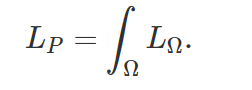
figure 4: we can also use Monte Carlo integration to approximate how much light arrives on a point.

remember from the lesson on shading, that Ω denotes the hemisphere. as usual though, this involves to integrate some quantity over a continous area, to which where is no analytical solution. thus, here again we can use a Monte Carlo integration method. this idea is to “sample” the hemisphere by creating on its surface random samples and shooting rays in the scene from P through these samples, to get an approximation of how much light arrives at P (figure 4). in other words, we cast random rays from the visible point P and average their result.

again, this is how a Monte Carlo ray tracer typically works. note that when we cast a ray from P into the scene to find out how much light comes from that direction, if we intersect another object along this ray, we use the same method to approximate the amount of light returned by this object. the procedure is recursive. because we follow the path of rays, this algorithm is also sometimes called path tracing. u can see it illustrated in figure 5.

this idea can also be expressed with the following pseudocode.

Vec3f monteCarloIntegration(P, N) 
{ 
    Vec3f lightAtP = 0; 
    int nsamples = 8; 
    for (int n = 0; n < nsamples; ++n) { 
        Ray sampleRay = sampleRayAboveHemisphere(P, N); 
        Vec3f Phit; 
        Vec3f Nhit; 
        if (traceRay(sampleRay, Phit, Nhit)) { 
            lightAtP += monteCarloIntegration(Phit, Nhit); 
        } 
    } 
    lightAtP /= nsamples; 
 
     return lightAtP; 
} 
 
void render() 
{ 
    Ray r; 
    computeCameraRayDir(r, ...); 
    Vec3f Phit; 
    Vec3f Nhit; 
    if (traceRay(r, Phit, Nhit)) { 
        Vec3f lightAtP = monteCarloIntegration(Phit, Nhit); 
        ... 
    } 
} 

we will study this algorithm in detail in the lesson on path tracing.

obviously, all that is a very quick and approximate (so to speak) introduction to Monte Carlo ray tracing. to get a more accurate and complete information we strongly advise u to read the rest of this lesson, and the following one.

to conclude though, let us say that Monte Carlo methods are numerical techniques relying on random sampling to approximate results, notably the results of integrals. these integrals can sometimes be resolved using other techniques (if u are interested, u can search for example for Las Vegas algorithms), however we will show in the next lessons that they have properties compared to other solutions which are making them more useful (especially to solve the sort of integrals we have to deal with in computer graphics).

Monte Carlo is aboslutely central to the field of rendering. it is connected to many very important other topics such sampling, importance sampling, light transport algorithms, and is also used in many other important rendering techniques (especially in shading).