KannalaBrandt8鱼眼相机模型

瞻邈

已于 2024-12-24 10:49:45 修改

阅读量4.1k

点赞数 6

分类专栏：计算机视觉文章标签：计算机视觉自动驾驶

于 2022-08-18 20:57:46 首次发布

本文链接：https://blog.csdn.net/xhtchina/article/details/126115380

版权

计算机视觉专栏收录该内容

8 篇文章

订阅专栏

1. 鱼眼相机

鱼眼相机镜头是由十几个不同的透镜组合而成，在成像的过程中，入射光线经过不同程度的折射，投影到尺寸有限的成像平面上，使得鱼眼镜头拥有更大的视野范围。下图为鱼眼相机的组成结构：

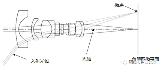
与针孔相机原理不同，鱼眼镜头采用非相似成像，在成像过程中引入畸变，通过对直径空间的压缩，突破成像视角的局限，从而达到广角成像。

鱼眼相机是一种焦距小于等于16mm，且视角接近或者等于180°的极端广角镜头，但是正是因为他极端的短焦和广角，导致它因为光学原理而产生的畸变非常剧烈，所以针孔模型并不能很好的描述鱼眼相机，所以需要一种新的相机模型来对鱼眼相机进行近似模拟。

2. 相机畸变

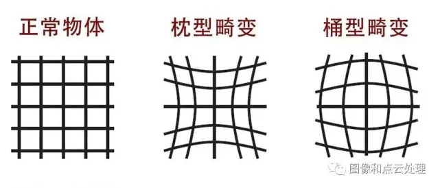
鱼眼镜头无论如何它的边缘线条都是要弯曲的，即使90度的鱼眼也是这样，这种畸变我们在很多广角镜头上都可以看到，而这就是明显的桶形畸变。同样的120度的鱼眼看起来弯曲的更加厉害一些了，而且被容纳进范围的景物更多；150度同样如此，而180度的鱼眼则可以把镜头周围180度范围内的所有物体都拍摄进去。众所周知，焦距越短，视角越大，因光学原理产生的变形也就越强烈。为了达到180度的超大视角，鱼眼镜头不得不允许这种变形（桶形畸变）的合理存在。

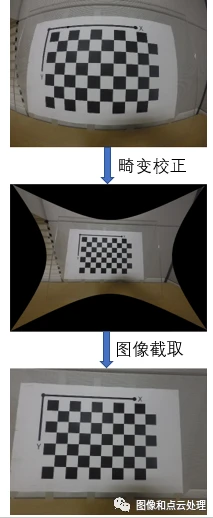
针对原始图像进行畸变校正后，带有冗余边界，需要做进一步截取。如下图：

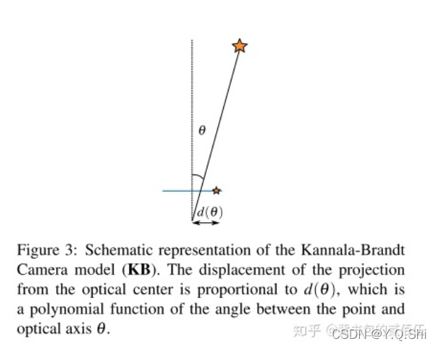
3. KannalaBrandt8模型

KB模型能够很好的适用于普通，广角以及鱼眼镜头。KB模型假设图像光心到投影点的距离和角度的多项式存在比例关系，角度的定义是点所在的投影光纤和主轴之间的夹角。

3.1. 投影过程

$u = f_x r cos(\phi) + c_x$

$v = f_y r sin(\phi) + c_y$

其中

$\theta = atan(\frac{\sqrt{x^2 + y^2}}{z})$

$r = \theta + k_1 \theta^3 + k_2 \theta^5 + k_3 \theta^7 + k_4 \theta^9$

$\phi = atan(\frac{y}{x})$

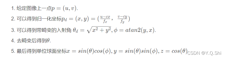
3.2. 反投影过程

4. KannalaBrandt8算法在ORB-SLAM3的实现

4.1. 投影

/**
  * @brief 投影
  * @param 3D点
  * @return 像素坐标
  * 注意：ORBSLAM3为投影重载了许多方法以接受各种不同的数据类型，在此就不一一列举了
  * 它们只是进行了数据类型之间的转换，然后统一以本方式实现，不再赘述
 **/
cv::Point2f KannalaBrandt8::project(const cv::Point3f &p3D)
{
	// r^2 = x^2 + y^2
    const float x2_plus_y2 = p3D.x * p3D.x + p3D.y * p3D.y;
    // θ = atan2(r,z) 
    const float theta = atan2f(sqrtf(x2_plus_y2), p3D.z);
    
    const float psi = atan2f(p3D.y, p3D.x);

	// 计算θ的3，5，7，9次方
	// 计算2次方是为了方便计算3，5，7，9次 相当于中间变量
    const float theta2 = theta * theta;
    const float theta3 = theta * theta2;
    const float theta5 = theta3 * theta2;
    const float theta7 = theta5 * theta2;
    const float theta9 = theta7 * theta2;
    // mvParameters是存放相机参数和畸变系数的数组
    // [4] [5] [6] [7] 分别代表k1 k2 k3 k4
    // 是不是感觉很熟悉 其实KB模型也常被用于针孔的畸变模型
    // 计算获得d(θ)
    const float r = theta + mvParameters[4] * theta3 + mvParameters[5] * theta5 + mvParameters[6] * theta7 + mvParameters[7] * theta9;
    // 注意：注释的r和代码的r不是一个东西 代码r = 注释d(θ) 注释r = 代码x2_plus_y2 
	// [0] [1] [2] [3] 分别代表 fx fy cx cy
	// 利用公式 u = (fx * d(θ) * xc) / r 
	// 		    v = (fy * d(θ) * yc) / r
	// cos(psi) = xc/r  sin(psi) = yc/r  
    return cv::Point2f(mvParameters[0] * r * cos(psi) + mvParameters[2],
                        mvParameters[1] * r * sin(psi) + mvParameters[3]);
}

4.2. 反投影

/**
  * @brief 反投影过程
  * @param 像素坐标
  * @return 归一化坐标
  **/
cv::Point3f KannalaBrandt8::unproject(const cv::Point2f &p2D)
{
    //Use Newton method to solve for theta with good precision (err ~ e-6)
    // 使用Newton法来求解θ，获得了很好的效果
    // 获取归一化的x,y坐标
    // x = (u - cx) / fx
    // y = (v - cy) / fy
    cv::Point2f pw((p2D.x - mvParameters[2]) / mvParameters[0], (p2D.y - mvParameters[3]) / mvParameters[1]);  // xd   yd
    // 设置尺度为1
    float scale = 1.f;
    // xd = θd/r * xc   yd = θd/r * yc
    // xd^2 + yd^2 = (θd^2 / r^2) * (xc^2 + yc^2)
    // xc^2 + yc^2 = r^2
    // θ = (xd^2 + yd^2)^(1/2)
    float theta_d = sqrtf(pw.x * pw.x + pw.y * pw.y);  // sin(psi) = yc / r
    //确保θd在[-π,π]的范围内 
    theta_d = fminf(fmaxf(-CV_PI / 2.f, theta_d), CV_PI / 2.f);  // 不能超过180度

	// 已知θd 求解 θ
    if (theta_d > 1e-8)
    {
        //Compensate distortion iteratively
        float theta = theta_d;  // θ的初始值定为了θd
        // 开始迭代
        for (int j = 0; j < 10; j++)
        {
            float theta2 = theta * theta, 
                  theta4 = theta2 * theta2,
                  theta6 = theta4 * theta2,
                  theta8 = theta4 * theta4;
            float k0_theta2 = mvParameters[4] * theta2,
                  k1_theta4 = mvParameters[5] * theta4;
            float k2_theta6 = mvParameters[6] * theta6,
                  k3_theta8 = mvParameters[7] * theta8;
            // f(θ) = θ + k1 * θ^3 + k2 * θ^5 + k3 * θ^7 + k4 * θ^9
            // e(θ) = f(θ) - θd
            // 直接求解θ很难 所以通过求导优化的方法
            // 目标是优化获得e(θ) = 0对应的θ
            // e(θ)' = 1 + 3 * k1 * θ^2 + 5 * k2 * θ^4 + 7 * k3 * θ^6 + 9 * k4 * θ^8
            // δ(θ) = e(θ) / e(θ)' 修正量
            float theta_fix = (theta * (1 + k0_theta2 + k1_theta4 + k2_theta6 + k3_theta8) - theta_d) /
                                (1 + 3 * k0_theta2 + 5 * k1_theta4 + 7 * k2_theta6 + 9 * k3_theta8);
            // 进行修正
            theta = theta - theta_fix;
            // 如果更新量变得很小，表示接近最终值
            if (fabsf(theta_fix) < precision) 
                break;
        }
        //scale = theta - theta_d;
        // 求得tan(θ) / θd
        scale = std::tan(theta) / theta_d;
    }
	// 获取归一化坐标
    return cv::Point3f(pw.x * scale, pw.y * scale, 1.f);
}

4.3. 求解雅各比矩阵

/**
  * @breif 求解像素坐标关于三维点的雅各比矩阵
  * @param p3D 三维点
  * @return 雅各比矩阵[一个两行三列的矩阵] 
  **/
  
cv::Mat KannalaBrandt8::projectJac(const cv::Point3f &p3D)
{
    float x2 = p3D.x * p3D.x, y2 = p3D.y * p3D.y, z2 = p3D.z * p3D.z;
    float r2 = x2 + y2;
    float r = sqrt(r2);
    float r3 = r2 * r;
    float theta = atan2(r, p3D.z);

    float theta2 = theta * theta, theta3 = theta2 * theta;
    float theta4 = theta2 * theta2, theta5 = theta4 * theta;
    float theta6 = theta2 * theta4, theta7 = theta6 * theta;
    float theta8 = theta4 * theta4, theta9 = theta8 * theta;

    float f = theta + theta3 * mvParameters[4] + theta5 * mvParameters[5] + theta7 * mvParameters[6] +
                theta9 * mvParameters[7];
    float fd = 1 + 3 * mvParameters[4] * theta2 + 5 * mvParameters[5] * theta4 + 7 * mvParameters[6] * theta6 +
                9 * mvParameters[7] * theta8;
	// u = (fx * θd * x) / r + cx
	// v = (fy * θd * y) / r + cy
	// θd = θ + k1 * θ^3 + k2 * θ^5 + k3 * θ^7 + k4 * θ^9
	// θ = arctan(r,z)
	// r = (x^2 + y^2)^(1/2)
    cv::Mat Jac(2, 3, CV_32F);
    Jac.at<float>(0, 0) = mvParameters[0] * (fd * p3D.z * x2 / (r2 * (r2 + z2)) + f * y2 / r3);  // ∂u/∂x
    Jac.at<float>(1, 0) =
        mvParameters[1] * (fd * p3D.z * p3D.y * p3D.x / (r2 * (r2 + z2)) - f * p3D.y * p3D.x / r3);  // ∂v/∂x

    Jac.at<float>(0, 1) =
        mvParameters[0] * (fd * p3D.z * p3D.y * p3D.x / (r2 * (r2 + z2)) - f * p3D.y * p3D.x / r3);  // ∂u/∂y
    Jac.at<float>(1, 1) = mvParameters[1] * (fd * p3D.z * y2 / (r2 * (r2 + z2)) + f * x2 / r3);  // ∂v/∂y

    Jac.at<float>(0, 2) = -mvParameters[0] * fd * p3D.x / (r2 + z2);  // ∂u/∂z
    Jac.at<float>(1, 2) = -mvParameters[1] * fd * p3D.y / (r2 + z2);  // ∂v/∂z

    std::cout << "CV JAC: " << Jac << std::endl;

    return Jac.clone();
}