ETO：解决复杂工程问题的指数-三角优化算法

---

1.摘要

本文提出了一种创新的优化算法——指数-三角优化算法（ETO），它巧妙地结合了指数函数和三角函数。ETO算法设计上着重于探索与开发两个阶段的平衡，这是众多优化算法共同面临的挑战。通过整合多个随机和自适应变量，ETO算法在性能上相比现有算法实现了显著的提升。

2.算法原理

指数-三角优化算法通过运用指数和三角函数来调整搜索个体的位置，有效实现了探索与开发的平衡。此外，ETO的设计考虑到了处理复杂技术问题的需要，基于NFL理论强调了不同问题需求不同优化策略的重要性。ETO的结构简单，易于实施和调整参数，使其不仅在性能上优越，还在适应不同问题类型上具有极高的灵活性和适应性。

受限探索方法

受限搜索策略通过有限探索方法来优化搜索过程，减少计算资源和时间消耗，同时确保捕捉到最优解：
$$\begin{array}{rl}& C{E}_{i+1}=floor[2-2\times t\times (Max\_Iter-C{E}_i\times a)]+C{E}_i\\ & \\ & C{E}_i=floor\left(1+\frac{Max\_Iter}{b}\right)\end{array}$$

受限探索策略确定当前迭代的探索限制，随后更新搜索空间的上限和下限：
$$\begin{array}{c}U{p}_i=r_1\times \left(1-\frac{t}{Max\_Iter}\right)\times \left|r_2\times X_j^{best}-X_j^s\right|+X_j^{best}\\ Lo{w}_i=-r_1\times \left(1-\frac{t}{Max\_Iter}\right)\times \left|r_2\times X_j^{best}-X_j^s\right|+X_j^{best}\end{array}$$

探索阶段

优化过程中的探索阶段被细分为两个阶段，持续的迭代对于防止算法收敛至局部最优解至关重要：
$$X_{t+1}^{i,j}=\{\begin{array}{l}{X}_j^{best}+rand()\times {\alpha }_1\times \left|X_j^{best}-X_t^{ij}\right|\mathrm{if}{q}_1\le 0.5\\ \\ X_j^{best}-rand()\times {\alpha }_1\times \left|X_j^{best}-X_t^{ij}\right|\mathrm{if}{q}_1>0.5\end{array}$$

其中，参数$a_1$表述为：
$${\alpha }_1=3\times rand()\times \left(\frac{t}{\text{Max}\_Iter}-0.85\right)\times \exp \left(\frac{d_1}{d_2}-1\right)$$

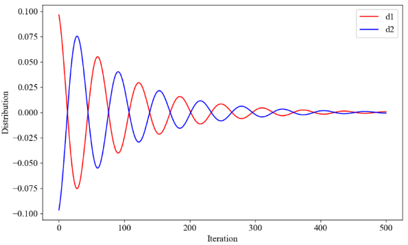
$$\begin{gathered} d_1=0.1\times \exp (-0.01\times t)\times \cos [0.5\times Ma{x}_{I}ter\times (1-\frac{t}{Ma{x}_{I}ter}\left)\right] \\ {d}_2=-0.1\times \exp (-0.01\times t)\times \cos [0.5\times Ma{x}_{I}ter\times (1-\frac{t}{Ma{x}_{I}ter}\left)\right] \end{gathered}$$

在探索程序的后续阶段，个体行为相对独立，不受之前确定的最佳解的影响。这种独立性使得它们可以无方向性偏见地进入搜索空间的新区域，其移动仅由当前位置直接决定。个体位置更新：
$$X_{t+1}^{ij}=\{\begin{array}{l}{X}_t^{ij}+3\times \left|rand()\times {\alpha }_2\times X_j^{best}-X_t^{ij}\right|\text{if}{q}_2\le 0.5\\ X_t^{ij}-3\times \left|rand()\times {\alpha }_2\times X_j^{best}-X_t^{ij}\right|\text{if}{q}_2>0.5\end{array}$$
其中，参数$a_2$表述为:
$${\alpha }_2=rand()\times \exp \left\{\tanh \left[1.5\times \left(-\frac{t}{Max\_Iter}-0.75\right)-rand()\right]\right\}$$

开发阶段

为确保全面探索搜索空间，开发过程被明确分为两个阶段，这两个阶段贯穿整个迭代过程。在第一阶段，算法主要集中于探索当前点邻域：
$$X_{t+1}^{ij}=\{\begin{array}{l}{X}_j^{best}+q_4\times {\alpha }_3\times \left|\mathbf{m}\mathbf{n}\mathbf{d}()\times X_j^{best}-X_t^{i,j}\right|\mathrm{if}{q}_3\le 0.5\\ X_j^{best}-q_4\times {\alpha }_3\times \left|\mathbf{m}\mathbf{n}\mathbf{d}()\times X_j^{best}-X_t^{i,j}\right|\mathrm{if}{q}_3>0.5\end{array}$$
其中，参数$a_3$表述为：
$${\alpha }_3=3\times rand()\times \left(\frac{t}{\text{Max}\_Iter}-0.85\right)\times \exp \left(\left|\frac{d_1}{d_2}\right|-1.3\right)$$

在开发的后期阶段，候选解中心围绕已识别的最佳解进行更集中的探索：
$$X_{t+1}^{ij}=X_t^{i,j}+c\times \left|rand()\times {\alpha }_2\times X_j^{best}-X_t^{i,j}\right|$$

其中，参数$c$表述为：
$$c=\exp \left[\tan \right(\left|\frac{d_1}{d_2}\right|\left)\right]$$

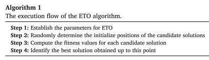
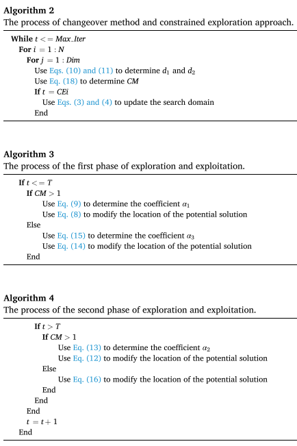
伪代码

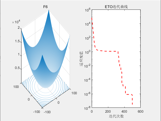
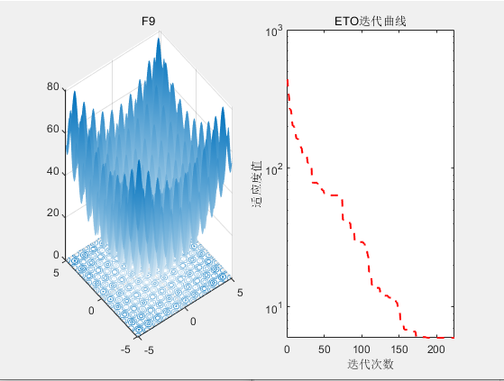
3.结果展示

4.参考文献

[1] Luan T M, Khatir S, Tran M T, et al. Exponential-trigonometric optimization algorithm for solving complicated engineering problems[J]. Computer Methods in Applied Mechanics and Engineering, 2024, 432: 117411.

5.代码获取