Homograph Matrix(单应性矩阵)、RANSAC(随机采样一致)及其在图像配准中的应用、代码讲解

写在前面

正在写…
1、文中所有资源、参考已给出来源链接，如有侵权请联系删除
2、本文实验环境：
win10+vs2019+opencv440(vs2019配置opencv+contrib-440 + PCL1.10.0 + 源码单步调试https://blog.csdn.net/qq_41102371/article/details/108727224)
visual studio opencv Mat可视化工具image watch：visual studio2019安装opencv可视化工具image watch https://blog.csdn.net/qq_41102371/article/details/116862557
3、为了尽量描述每个问题，文章内涉及分支较多，建议先整体阅读，想对某一块知识深究原理的再点击相应链接继续学习
4、码字不易，转载本文请注明出处，本文链接：https://blog.csdn.net/qq_41102371/article/details/116668677

使用单应性矩阵配准图像实验

原图来自opencv(\opencv-4.4.0\samples\data目录下)https://github.com/opencv/opencv/tree/master/samples/data
graf3.png（左图）graf3.png（右图）
求单应性矩阵并RANSAC剔除误匹配点后

使用单应性变换矩阵将右图配准至左图效果

图像配准原理、实现分析见这篇文章：
基于sift算法的图像配准、Homograph Matrix、RANSAC https://blog.csdn.net/qq_41102371/article/details/116031738
完整项目文件免费下载地址：
[share_noel/Opencv&Image Processing/202105image registration/202105image_registration.zip]https://blog.csdn.net/qq_41102371/article/details/125646840
愿意用c币支持的朋友也可在此下载：
202105image_registration.zip https://download.csdn.net/download/qq_41102371/18717986
（上述下载链接中csdn与网盘的文件完全相同，只不过网盘免费下载）

单应性矩阵

理解

可以用两种方式去理解，一直接从平面与平面之间的旋转、平移、缩放、透视变换出发去理解，在
1、基于sift算法的图像配准、Homograph Matrix、RANSAC https://blog.csdn.net/qq_41102371/article/details/116031738
2、图像旋转平移、仿射变换、透视变换 https://blog.csdn.net/qq_41102371/article/details/116245483
这两篇文章中有讲解
二是通过三维空间到二维平面的投影矩阵去理解
VSLAM中的X点法汇总https://zhuanlan.zhihu.com/p/103591977
（关于三维空间坐标变换以及三维到二维的投影变换见此文：待完成…）
假设所有点位于同一个平面并且设这个平面为$Z=0$，于是将3D到2D的变换模型简化成了空间中平面到平面的单应性变换
$$s\left[\begin{array}{c}u\\ v\\ 1\end{array}\right]=K\left[\begin{array}{cccc}{r}_1& r_2& r_3& t\end{array}\right]\left[\begin{array}{c}X\\ Y\\ 0\\ 1\end{array}\right]=K\left[\begin{array}{ccc}{r}_1& r_2& t\end{array}\right]\left[\begin{array}{c}X\\ Y\\ 1\end{array}\right]=H\left[\begin{array}{c}X\\ Y\\ 1\end{array}\right]$$
其中
$$H=\left[\begin{array}{ccc}{h}_{11}& h_{12}& h_{13}\\ h_{21}& h_{22}& h_{23}\\ h_{31}& h_{32}& h_{33}\end{array}\right]$$
就是单应性变换矩阵,$s$是一个任意大小的尺度因子
于是有
$$\begin{array}{rl}s\ast u& =h_{11}X+h_{12}Y+h_{13}\\ s\ast v& =h_{21}X+h_{22}Y+h_{23}\\ s& =h_{31}X+h_{32}Y+h_{33}\end{array}$$
消去$s$
$$\Rightarrow \begin{array}{rl}u& =\frac{h_{11}X+h_{12}Y+h_{13}}{h_{31}X+h_{32}Y+h_{33}}\\ v& =\frac{h_{21}X+h_{22}Y+h_{23}}{h_{31}X+h_{32}Y+h_{33}}\end{array}$$

求解推导

用二维点$(x_i^{\prime },y_i^{\prime })$表示图像坐标$(u,v)$，用$(x_i,y_i)$表示三维平面$Z=0$上的点$(X,Y)$，整理得：
$$\Rightarrow \begin{array}{rl}-x_i\ast h_{11}-y_i\ast h_{12}-1\ast h_{13}+0\ast h_{21}+0\ast h22+0\ast h_{23}+x_i\ast x_i^{\prime }\ast h_{31}+y_i\ast x_i^{\prime }\ast h_{32}+x_i^{\prime }\ast h_{33}& =0\\ 0\ast h_{11}+0\ast h_{12}+0\ast h_{13}-x_i\ast h_{21}-y_i\ast h22-1\ast h_{23}+x_i\ast y_i^{\prime }\ast h_{31}+y_i\ast y_i^{\prime }\ast h_{32}+y_i^{\prime }\ast h_{33}& =0\end{array}$$
写成矩阵：
$$\left[\begin{array}{ccccccccc}-x_i& -y_i& -1& 0& 0& 0& x_i{x}_i^{\prime }& y_i{x}_i^{\prime }& x_i^{\prime }\\ 0& 0& 0& -x_i& -y_i& -1& x_i{y}_i^{\prime }& y_i{y}_i^{\prime }& y_i^{\prime }\end{array}\right]\left[\begin{array}{c}{h}_{11}\\ h_{12}\\ h_{13}\\ h_{21}\\ h_{22}\\ h_{23}\\ h_{31}\\ h_{32}\\ h_{33}\end{array}\right]=0$$
令$h=\left[\begin{array}{ccccccccc}{h}_{11}& h_{12}& h_{13}& h_{21}& h_{22}& h_{23}& h_{31}& h_{32}& h_{33}\end{array}\right]$:
$$\left[\begin{array}{ccccccccc}-x_i& -y_i& -1& 0& 0& 0& x_i{x}_i^{\prime }& y_i{x}_i^{\prime }& x_i^{\prime }\\ 0& 0& 0& -x_i& -y_i& -1& x_i{y}_i^{\prime }& y_i{y}_i^{\prime }& y_i^{\prime }\end{array}\right]h=0$$

$h$相当于是将$H$展成了一维向量，当我们使用特征检测、匹配、误匹配剔除后，相当于知道了两平面的对应点对$(x_i,y_i)$与$(x_i^{\prime },y_i^{\prime })$，那么上式就是方程组求解的问题，$h$一共9个未知数，每组点对提供两个方程，需要至少5对点才能解出方程；我们回到前面说的尺度因子$s$：
$$s\left[\begin{array}{c}{x}_i^{\prime }\\ y_i^{\prime }\\ 1\end{array}\right]=H\left[\begin{array}{c}x\\ y\\ 1\end{array}\right]$$
其实单应性矩阵$H$与$\alpha H$一样（其中$\alpha \ne 0$），令$\alpha =\frac{1}{s}$，左右两边乘以$\alpha$
$$\left[\begin{array}{c}{x}_i^{\prime }\\ y_i^{\prime }\\ 1\end{array}\right]=\alpha H\left[\begin{array}{c}x\\ y\\ 1\end{array}\right]$$
$$\Rightarrow \begin{array}{rl}{x}_i^{\prime }& =\frac{\alpha h_{11}{x}_i+\alpha h_{12}{y}_i+\alpha h_{13}}{\alpha h_{31}{x}_i+\alpha h_{32}{y}_i+\alpha h_{33}}=\frac{h_{11}{x}_i+h_{12}{y}_i+h_{13}}{h_{31}{x}_i+h_{32}{y}_i+h_{33}}\\ y_i^{\prime }& =\frac{\alpha h_{21}{x}_i+\alpha h_{22}{y}_i+\alpha h_{23}}{\alpha h_{31}{x}_i+\alpha h_{32}{y}_i+\alpha h_{33}}=\frac{h_{21}{x}_i+h_{22}{y}_i+h_{23}}{h_{31}{x}_i+h_{32}{y}_i+h_{33}}\end{array}$$
所以无论是$H$还是$\alpha H$，变换之后都是$(x_i^{\prime },y_i^{\prime })$，如果再令$\alpha =\frac{1}{h_{33}}$，那么:
$$H=\left[\begin{array}{ccc}{h}_{11}& h_{12}& h_{13}\\ h_{21}& h_{22}& h_{23}\\ h_{31}& h_{32}& h_{33}\end{array}\right]=\frac{1}{h_{33}}H=\left[\begin{array}{ccc}\frac{h_{11}}{h_{33}}& \frac{h_{12}}{h_{33}}& \frac{h_{13}}{h_{33}}\\ \frac{h_{21}}{h_{33}}& \frac{h_{22}}{h_{33}}& \frac{h_{23}}{h_{33}}\\ \frac{h_{31}}{h_{33}}& \frac{h_{32}}{h_{33}}& 1\end{array}\right]$$
于是有，
$$\left[\begin{array}{c}{x}_i^{\prime }\\ y_i^{\prime }\\ 1\end{array}\right]=H\left[\begin{array}{c}x\\ y\\ 1\end{array}\right]$$
其中$h_{33}=1$
（单应性Homograph估计：从传统算法到深度学习https://zhuanlan.zhihu.com/p/74597564）
因此$H$矩阵虽然是9个未知数，但是由于尺度因子的存在，可以令$h_{33}=1$，于是单应性矩阵只有8个自由度。所以如果有4组不共线的对应点对，就可以求出方程的唯一解，但是由于噪声的存在，一般会使用多于4组点对来求解，当方程组个数多于未知数个数时，就是超定方程组的问题，可以用最小二乘求解，即：
$$\left[\begin{array}{ccccccccc}-x_i& -y_i& -1& 0& 0& 0& x_i{x}_i^{\prime }& y_i{x}_i^{\prime }& x_i^{\prime }\\ 0& 0& 0& -x_i& -y_i& -1& x_i{y}_i^{\prime }& y_i{y}_i^{\prime }& y_i^{\prime }\\ ...& & & & & & & & \end{array}\right]\left[\begin{array}{c}{h}_{11}\\ h_{12}\\ h_{13}\\ h_{21}\\ h_{22}\\ h_{23}\\ h_{31}\\ h_{32}\\ h_{33}\end{array}\right]=\left[\begin{array}{c}0\\ 0\\ ...\\ \\ \\ \\ \\ \\ \end{array}\right]\Rightarrow Ax=0$$
（单应性矩阵的理解及求解https://blog.csdn.net/liubing8609/article/details/85340015）
其中$A$是$N\times 2$的矩阵，$N$是点对数量，每个点对提供2个方程，因此$N$个点对就构成$N\times 2$的矩阵，$x$就是要求解的$h$。关于为什么最小二乘的解是超定线性方程组的解，在这几篇文章中有详细的推导说明：
超定方程的求解、最小二乘解、Ax=0、Ax=b的解，求解齐次方程组，求解非齐次方程组（推导十分详细） https://blog.csdn.net/u011341856/article/details/107758182
证明Ax=0的最小二乘解是ATA的最小特征值对应的特征向量(||x||＝1) https://blog.csdn.net/baidu_38172402/article/details/89520326
特征值 是 系数行列式等于0时的 解
正交矩阵的保范性:正交变换不改变向量的长度(范数)https://blog.csdn.net/qq_33898609/article/details/105734389
L1范数与L2范数的区别https://blog.csdn.net/rocling/article/details/90290576
什么是范数（norm）？以及L1,L2范数的简单介绍https://blog.csdn.net/qq_37466121/article/details/87855185
如何让奇异值分解(SVD)变得不“奇异”？http://redstonewill.com/1529/
记住比较重要的结论：
超定方程$Ax=0$的解，就是对 $A$进行SVD分解之后的最小特征值对应的特征向量。
或者说：最小特征值对应的特征向量是最小二乘的解
另外，因为$H$矩阵是可以乘以任意系数的，那么怎么保证我们求解出来唯一的解呢，一般是将$h$的模值限定为1:
$$h_{11}^2+h_{12}^2+h_{13}^2+h_{21}^2+h_{22}^2+h_{23}^2+h_{31}^2+h_{32}^2+h_{33}^2=1$$
也就是$Ax=0$中$\Vert x\Vert =1$，同时这也对应着:当 $\Vert x\Vert =1$时，Ax=0的最小二乘解是$A^{T}A$的最小特征值对应的特征向量(证明Ax=0的最小二乘解是ATA的最小特征值对应的特征向量(||x||＝1) https://blog.csdn.net/baidu_38172402/article/details/89520326)

误差剔除与RANSAC

实际特征点检测、匹配并不是完美的，因此可能会带来误差、误匹配，而最小二乘是从一个整体误差最小的角度去考虑，是非常容易受噪声影响的（噪声属于整体的一部分），因此需要使用随机采样一致性算法(Random sample consensus，RANSAC）来保留最优的数据：
计算机视觉基本原理——RANSAC https://zhuanlan.zhihu.com/p/45532306
随机抽样一致算法（Random sample consensus，RANSAC） https://www.cnblogs.com/xingshansi/p/6763668.html
对于RANSAC，最简单的理解方法就是少数服从多数：总共m个数据，设定一个误差k，选取模型最低需要的数据个数求解，如果求解出的模型H能使其余n个数据在给定误差范围k内，服从这个模型（内点），并且与其他求解出的模型相比，H对应的n是最大的。比如现在有100个点对，homography矩阵需要至少4个点对，假如总共迭代三次，每次选出的点对集合为$P_i$，求解出的模型为$H_i$，将求解到的模型应用到其他数据，误差小于k的视为内点，假设结果如下：

集合	模型	内点数
$P_1$	$H_1$	90
$P_2$	$H_2$	20
$P_3$	$H_3$	10
很显然，对于集合$P_1$求解出的模型，在100对点对中有90对点对是在误差内符合这个模型的，因此最终以$H_1$作为最优的结果，并且使用这90个点对重新去求解一个更精确的模型。后面将结合代码的讲解来理解RANSAC。

opencv源码讲解

本源码讲解在文章开头的环境配置的基础之上，工程文件上文已给出免费下载地址

函数接口

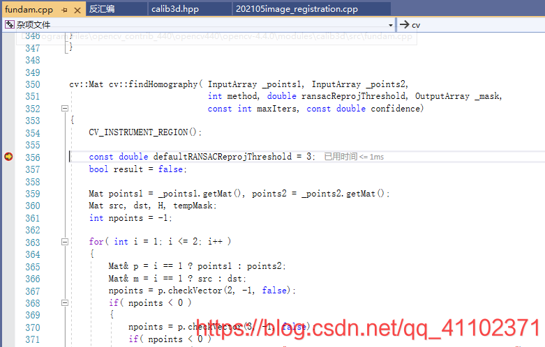
findHomography()函数在\opencv-4.4.0\modules\calib3d\src\fundam.cpp line:350

Mat cv::findHomography	(
InputArray 	srcPoints,
InputArray 	dstPoints,
int 	method = 0,
double 	ransacReprojThreshold = 3,
OutputArray 	mask = noArray(),
const int 	maxIters = 2000,
const double 	confidence = 0.995 
)	

本文使用opencv提供的单应性矩阵求解函数，opencv的官方文档中有对函数接口的解释以及单应性变换的描述
opencv官方文档findHomography–https://docs.opencv.org/4.4.0/d9/d0c/group__calib3d.html#ga4abc2ece9fab9398f2e560d53c8c9780
Finds a perspective transformation between two planes.
Parameters
srcPoints：Coordinates of the points in the original plane, a matrix of the type CV_32FC2 or vector<Point2f> .
dstPoints: Coordinates of the points in the target plane, a matrix of the type CV_32FC2 or a vector<Point2f> .
method: Method used to compute a homography matrix. The following methods are possible:

• 0 - a regular method using all the points, i.e., the least squares method
• RANSAC - RANSAC-based robust method
• LMEDS - Least-Median robust method
• RHO - PROSAC-based robust method
  ransacReprojThreshold: Maximum allowed reprojection error to treat a point pair as an inlier (used in the RANSAC and RHO methods only). That is, if
  $$\Vert {\text{dstPoints}}_i-\text{convertPointsHomogeneous}(\text{H}\ast {\text{srcPoints}}_i){\Vert }_2>\text{ransacReprojThreshold}$$
  then the point i is considered as an outlier. If srcPoints and dstPoints are measured in pixels, it usually makes sense to set this parameter somewhere in the range of 1 to 10.
  mask: Optional output mask set by a robust method ( RANSAC or LMEDS ). Note that the input mask values are ignored.
  maxIters: The maximum number of RANSAC iterations.
  confidence: Confidence level, between 0 and 1.
  The function finds and returns the perspective transformation $H$ between the source and the destination planes:
  $$\left[\begin{array}{c}{x}_i^{\prime }\\ y_i^{\prime }\\ 1\end{array}\right]\sim H\left[\begin{array}{c}{x}_i\\ y_i\\ 1\end{array}\right]$$
  so that the back-projection error
  $$\sum _i{\left(x_i^{\prime }-\frac{h_{11}{x}_i+h_{12}{y}_i+h_{13}}{h_{31}{x}_i+h_{32}{y}_i+h_{33}}\right)}^2+{\left(y_i^{\prime }-\frac{h_{21}{x}_i+h_{22}{y}_i+h_{23}}{h_{31}{x}_i+h_{32}{y}_i+h_{33}}\right)}^2$$
  is minimized. If the parameter method is set to the default value 0, the function uses all the point pairs to compute an initial homography estimate with a simple least-squares scheme.

However, if not all of the point pairs ( $srcPoint{s}_i,dstPoint{s}_i$ ) fit the rigid perspective transformation (that is, there are some outliers), this initial estimate will be poor. In this case, you can use one of the three robust methods. The methods RANSAC, LMeDS and RHO try many different random subsets of the corresponding point pairs (of four pairs each, collinear pairs are discarded), estimate the homography matrix using this subset and a simple least-squares algorithm, and then compute the quality/goodness of the computed homography (which is the number of inliers for RANSAC or the least median re-projection error for LMeDS). The best subset is then used to produce the initial estimate of the homography matrix and the mask of inliers/outliers.

Regardless of the method, robust or not, the computed homography matrix is refined further (using inliers only in case of a robust method) with the Levenberg-Marquardt method to reduce the re-projection error even more.

The methods RANSAC and RHO can handle practically any ratio of outliers but need a threshold to distinguish inliers from outliers. The method LMeDS does not need any threshold but it works correctly only when there are more than 50% of inliers. Finally, if there are no outliers and the noise is rather small, use the default method (method=0).

The function is used to find initial intrinsic and extrinsic matrices. Homography matrix is determined up to a scale. Thus, it is normalized so that h33=1. Note that whenever an $H$ matrix cannot be estimated, an empty one will be returned.

函数作用是求出两个平面之间的透视变换
参数
srcPoints：源平面的的特征点坐标，数据类型为CV_32FC2的mat或者vector<Point2f>-----(m.x, m.y)
dstPoints：目标平面的的特征点坐标，数据类型为CV_32FC2的mat或者vector<Point2f>-----(m.x, m.y)
method:优化方法

• 0 - 所有点对都参与运算的常规方法—最小二乘法
• RANSAC - 基于RANSAC算法的鲁棒方法
• RHO - 基于PROSAC的鲁棒方法（这个没接触过）
  ransacReprojThreshold：（使用RANSAC和RHO时有效）最大允许重投影误差，默认为3个像素；重投影误差小于ransacReprojThreshold的为内点，大于的为外点，即
  $$\Vert {\text{dstPoints}}_i-\text{convertPointsHomogeneous}(\text{H}\ast {\text{srcPoints}}_i){\Vert }_2>\text{ransacReprojThreshold}$$

若源点与目标点都是以像素为度量的，通常此参数设置为1-10都可以。
mask：掩膜矩阵，由鲁棒方法（RANSAC或LMEDS）设定，注意输入的掩膜矩阵将被忽略（也就是自己输入空的掩膜mat和带值的掩膜mat都一样，会返回算出来的掩膜，输入带值的mat对算法不起作用）
maxIters：RANSAC算法的最大迭代次数
confidence：置信度，0-1之间
函数返回一个源源平面和目标平面之间的透视变换矩阵$H$
$$\left[\begin{array}{c}{x}_i^{\prime }\\ y_i^{\prime }\\ 1\end{array}\right]\sim H\left[\begin{array}{c}{x}_i\\ y_i\\ 1\end{array}\right]$$
矩阵$H$让反投影误差
$$\sum _i{\left(x_i^{\prime }-\frac{h_{11}{x}_i+h_{12}{y}_i+h_{13}}{h_{31}{x}_i+h_{32}{y}_i+h_{33}}\right)}^2+{\left(y_i^{\prime }-\frac{h_{21}{x}_i+h_{22}{y}_i+h_{23}}{h_{31}{x}_i+h_{32}{y}_i+h_{33}}\right)}^2$$
最小。如果method参数被设置为0，函数将使用最小二乘方法来计算比较初步的单应性矩阵，因为最小二乘方法是让所有的点参与运算，当某些点对是误匹配点对，即这些点对不满足刚体的透视变换时，这种初步的估计将会效果很差。
RANSAC, LMeDS and RHO方法会尝试很多的子点对集（非共线的四点对集），在这些子集上运用最小二乘来估计单应性矩阵，并计算出所得单应性矩阵的质量/好坏(RANSAC的内点数量或者最小中值法的最小中值重投影误差)。最好的子集将会用来产生初步的单应性矩阵的估计并生成掩膜矩阵。
不管使用哪种方法来计算初步的单应性矩阵，接着都会使用Levenberg-Marquardt（列文伯格-马夸尔特）方法来进一步优化(当使用鲁棒方法时，至使用内点进行计算)，以此进一步减少重投影误差。
RANSAC and RHO可以处理任意比例的离群值，但是需要一个阈值来分辨内点和外点。LMeDS 不需要阈值，但是仅能在内点数超过50%的情况下正确工作。最后，如果没有外点或者噪声很少，可以用默认的方法(method=0，最小二乘方法)。
此函数常用来求解内外参矩阵，单应性矩阵一个尺度差异，因此通常设置h33=1.注意当$H$矩不能被估计时，将返回一个空矩阵。

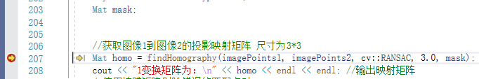
使用

单应性矩阵的调用如下，输入参数为对应点对，优化方法使用RANSAC，重投影误差为3个像素，mask掩膜矩阵

	Mat mask;
    Mat homo = findHomography(imagePoints1, imagePoints2, cv::RANSAC, 3.0, mask);

调试

运行代码，在findHomography()函数处加入断点

F11进入函数，函数在\opencv-4.4.0\modules\calib3d\src\fundam.cpp line:350

下面将进行部分代码的注释

核心代码1：findHomography的接口

cv::Mat cv::findHomography( InputArray _points1, InputArray _points2,
                            int method, double ransacReprojThreshold, OutputArray _mask,
                            const int maxIters, const double confidence)
{
    CV_INSTRUMENT_REGION();
	//重投影误差默认为3，后面会用到
    const double defaultRANSACReprojThreshold = 3;
    bool result = false;

    Mat points1 = _points1.getMat(), points2 = _points2.getMat();
    Mat src, dst, H, tempMask;
    int npoints = -1;
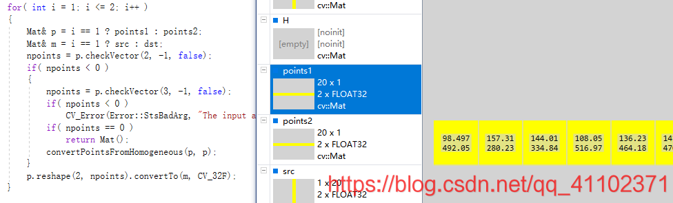
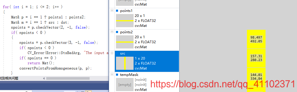
	//将输入的点矩阵更改排列方式，方便后面使用，见图p1和p2
    for( int i = 1; i <= 2; i++ )
    {
        Mat& p = i == 1 ? points1 : points2;
        Mat& m = i == 1 ? src : dst;
        npoints = p.checkVector(2, -1, false);
        if( npoints < 0 )
        {
            npoints = p.checkVector(3, -1, false);
            if( npoints < 0 )
                CV_Error(Error::StsBadArg, "The input arrays should be 2D or 3D point sets");
            if( npoints == 0 )
                return Mat();
            convertPointsFromHomogeneous(p, p);
        }
        p.reshape(2, npoints).convertTo(m, CV_32F);
    }

    CV_Assert( src.checkVector(2) == dst.checkVector(2) );
	//判断传入的重投影误差是否小于0，如果是的话重置为默认值3.0
    if( ransacReprojThreshold <= 0 )
        ransacReprojThreshold = defaultRANSACReprojThreshold;

    Ptr<PointSetRegistrator::Callback> cb = makePtr<HomographyEstimatorCallback>();
	//如果优化方法参数为0或者只有4对点对，那么直接使用最小二乘求解
    if( method == 0 || npoints == 4 )
    {
        tempMask = Mat::ones(npoints, 1, CV_8U);
        result = cb->runKernel(src, dst, H) > 0;
    }
    //使用RANSAC，创建RANSAC对象，见核心代码2，并运行run()函数，见核心代码3：ransac run()函数
    else if( method == RANSAC )
        result = createRANSACPointSetRegistrator(cb, 4, ransacReprojThreshold, confidence, maxIters)->run(src, dst, H, tempMask);
    else if( method == LMEDS )
        result = createLMeDSPointSetRegistrator(cb, 4, confidence, maxIters)->run(src, dst, H, tempMask);
    else if( method == RHO )
        result = createAndRunRHORegistrator(confidence, maxIters, ransacReprojThreshold, npoints, src, dst, H, tempMask);
    else
        CV_Error(Error::StsBadArg, "Unknown estimation method");
	//如果创建成功&&点对数大于4&&优化方法不是RHO
    if( result && npoints > 4 && method != RHO)
    {
        compressElems( src.ptr<Point2f>(), tempMask.ptr<uchar>(), 1, npoints );
        //根据掩膜矩阵计算内点个数
        npoints = compressElems( dst.ptr<Point2f>(), tempMask.ptr<uchar>(), 1, npoints );
        if( npoints > 0 )
        {
            Mat src1 = src.rowRange(0, npoints);
            Mat dst1 = dst.rowRange(0, npoints);
            src = src1;
            dst = dst1;
            //使用所有内点和最小二乘来重新计算模型
            if( method == RANSAC || method == LMEDS )
                cb->runKernel( src, dst, H );
            Mat H8(8, 1, CV_64F, H.ptr<double>());
            //使用列文伯格马夸尔特方法优化结果
            LMSolver::create(makePtr<HomographyRefineCallback>(src, dst), 10)->run(H8);
        }
    }

    if( result )
    {
        if( _mask.needed() )
            tempMask.copyTo(_mask);
    }
    else
    {
        H.release();
        if(_mask.needed() ) {
            tempMask = Mat::zeros(npoints >= 0 ? npoints : 0, 1, CV_8U);
            tempMask.copyTo(_mask);
        }
    }
	//返回最终的单应性矩阵
    return H;
}

图p1

图p2

核心代码2：创建RANSAC对象

opencv440\opencv-4.4.0\modules\calib3d\src\ptsetreg.cpp line:375

Ptr<PointSetRegistrator> createRANSACPointSetRegistrator(const Ptr<PointSetRegistrator::Callback>& _cb,
                                                         int _modelPoints, double _threshold,
                                                         double _confidence, int _maxIters)
{
	//创建一个RANSAC处理对象，初始化模型点数、重投影阈值、置信度、最大迭代次数等参数，返回创建的RANSAC对象
    return Ptr<PointSetRegistrator>(
        new RANSACPointSetRegistrator(_cb, _modelPoints, _threshold, _confidence, _maxIters));
}

核心代码3：ransac run()函数

opencv440\opencv-4.4.0\modules\calib3d\src\ptsetreg.cpp line:158

bool run(InputArray _m1, InputArray _m2, OutputArray _model, OutputArray _mask) const CV_OVERRIDE
    {
    	//函数返回的bool变量
        bool result = false;
        //点对
        Mat m1 = _m1.getMat(), m2 = _m2.getMat();
        //重投影误差（对应每个点对）、掩膜矩阵、
        //当前模型、当前最好的模型、随机选取的4组点对用于求解模型
        Mat err, mask, model, bestModel, ms1, ms2;
		//迭代次数
        int iter, niters = MAX(maxIters, 1);
        int d1 = m1.channels() > 1 ? m1.channels() : m1.cols;
        int d2 = m2.channels() > 1 ? m2.channels() : m2.cols;
        int count = m1.checkVector(d1), count2 = m2.checkVector(d2), maxGoodCount = 0;
		//产生随机数https://blog.csdn.net/gdfsg/article/details/50830489
        RNG rng((uint64)-1);

        CV_Assert( cb );
        CV_Assert( confidence > 0 && confidence < 1 );

        CV_Assert( count >= 0 && count2 == count );
        //判断点对数是否小于模型求解最少需要的数量
        if( count < modelPoints )
            return false;
		//掩膜矩阵
        Mat bestMask0, bestMask;

        if( _mask.needed() )
        {
            _mask.create(count, 1, CV_8U, -1, true);
            bestMask0 = bestMask = _mask.getMat();
            CV_Assert( (bestMask.cols == 1 || bestMask.rows == 1) && (int)bestMask.total() == count );
        }
        else
        {
            bestMask.create(count, 1, CV_8U);
            bestMask0 = bestMask;
        }
		//如果传入的点对数刚好等于模型求解需要的点对数，则直接使用最小二乘进行求解
        if( count == modelPoints )
        {
        	if( cb->runKernel(m1, m2, bestModel) <= 0 )
                return false;
            bestModel.copyTo(_model);
            bestMask.setTo(Scalar::all(1));
            return true;
        }
		//开始RANSAC迭代，最开始niters是2000
        for( iter = 0; iter < niters; iter++ )
        {
            int i, nmodels;
            if( count > modelPoints )
            {
            	//随机选点对
                bool found = getSubset( m1, m2, ms1, ms2, rng, 10000 );
                if( !found )
                {
                    if( iter == 0 )
                        return false;
                    break;
                }
            }
			//使用随机选取的4对点对求解模型，模型结果放在model中，见核心代码4:最小二乘求解的SVD求解
            nmodels = cb->runKernel( ms1, ms2, model );
            
            if( nmodels <= 0 )
                continue;
            CV_Assert( model.rows % nmodels == 0 );
            Size modelSize(model.cols, model.rows/nmodels);

            for( i = 0; i < nmodels; i++ )
            {
                Mat model_i = model.rowRange( i*modelSize.height, (i+1)*modelSize.height );
                //根据重投影误差判断内点，生成mask掩膜矩阵
                int goodCount = findInliers( m1, m2, model_i, err, mask, threshold );
				//如果当次的内点数比之前的多
                if( goodCount > MAX(maxGoodCount, modelPoints-1) )
                {
                	//更新当前最优的掩膜矩阵
                    std::swap(mask, bestMask);
                    //更新当前最优的模型
                    model_i.copyTo(bestModel);
                    //更新当前的最优内点数
                    maxGoodCount = goodCount;
                    //更新RANSAC的迭代次数
                    //更新原理：RANSAC算法理解 https://blog.csdn.net/robinhjwy/article/details/79174914
                    niters = RANSACUpdateNumIters( confidence, (double)(count - goodCount)/count, modelPoints, niters );
                }
            }
        }

        if( maxGoodCount > 0 )
        {
            if( bestMask.data != bestMask0.data )
            {
                if( bestMask.size() == bestMask0.size() )
                    bestMask.copyTo(bestMask0);
                else
                    transpose(bestMask, bestMask0);
            }
            bestModel.copyTo(_model);
            result = true;
        }
        else
            _model.release();

        return result;
    }

在这里将一下具体的RANSAC，在求解单应性矩阵的时候至少需要4组点对，所以上述代码每次随机选择了4组点对，选取之后使用

cb->runKernel( ms1, ms2, model );

来算出当前4组点满足的单应性矩阵模型(model)$H_1$，接着使用这个模型去寻找所有点对中的内点，就是将src点使用$H_1$变换到dst点的平面，看每个投影后的点与对应的dst点距离是多少，如果满足设定的3个像素以内，那么说明是内点，假设此次内点数为$n_1$，并更新掩膜矩阵，掩膜矩阵就是将非内点标记为0，内点标记为1；
接着进行下一次迭代，也是随机选4组点，如果算出来新的模型$H_2$，如果满足$H_2$模型的内点数$n_2>n_1$那么就保留$H_2$作为当前最好的结果，掩膜矩阵也是，如果$n_2<n_1$那么不更新最好的模型、内点、以及掩膜矩阵；
继续迭代直到迭代次数超过阈值。
迭代次数是会在每次迭代过程中更新的，可能最开始设置的2000，实际上最后可能只会迭代几十次，关于迭代次数的更新原理，见：
RANSAC算法理解 https://blog.csdn.net/robinhjwy/article/details/79174914
RANSAC算法在图像拼接上的应用的实现https://blog.csdn.net/weixin_34001430/article/details/89613160
OpenCV中的RANSAC详解https://blog.csdn.net/laobai1015/article/details/51683076
RANSAC 算法详解https://www.cnblogs.com/weizc/p/5257496.html
RANSAC https://blog.csdn.net/weixin_45748803/article/details/102675635
深度解析RANSAC算法 https://blog.csdn.net/weixin_43795395/article/details/90751650
昨晚上又失眠了到两点过，还好，已经习惯了，我跟失眠已经和解了；
然后睡到自然醒------5点，躺了两小时没睡着，7点过了还是起床吧；
到实验室，把那几个矩阵变换想明白是为什么了，趁热写下来

核心代码4：最小二乘求解的SVD求解runKernel()

opencv440\opencv-4.4.0\modules\calib3d\src\fundam.cpp line:116

    /**
     * Normalization method:
     *  - $x$ and $y$ coordinates are normalized independently
     *  - first the coordinates are shifted so that the average coordinate is \f$(0,0)\f$
     *  - then the coordinates are scaled so that the average L1 norm is 1, i.e,
     *  the average L1 norm of the \f$x\f$ coordinates is 1 and the average
     *  L1 norm of the \f$y\f$ coordinates is also 1.
     *
     * @param _m1 source points containing (X,Y), depth is CV_32F with 1 column 2 channels or
     *            2 columns 1 channel
     * @param _m2 destination points containing (x,y), depth is CV_32F with 1 column 2 channels or
     *            2 columns 1 channel
     * @param _model, CV_64FC1, 3x3, normalized, i.e., the last element is 1
     */

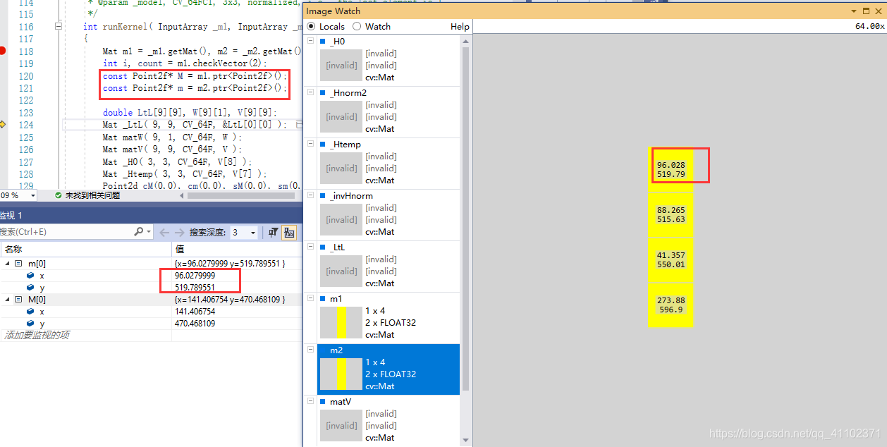
 int runKernel( InputArray _m1, InputArray _m2, OutputArray _model ) const CV_OVERRIDE
    {	//输入转成mat
        Mat m1 = _m1.getMat(), m2 = _m2.getMat();
        //count是点对的数量，正常就该为4
        int i, count = m1.checkVector(2);
        //将mat里面的点转成Point2f，也就是(x,y)形式，方便后面的计算使用
        const Point2f* M = m1.ptr<Point2f>();
        const Point2f* m = m2.ptr<Point2f>();
		
        double LtL[9][9], W[9][1], V[9][9];
        Mat _LtL( 9, 9, CV_64F, &LtL[0][0] );
        Mat matW( 9, 1, CV_64F, W );
        Mat matV( 9, 9, CV_64F, V );
        Mat _H0( 3, 3, CV_64F, V[8] );
        Mat _Htemp( 3, 3, CV_64F, V[7] );
        Point2d cM(0,0), cm(0,0), sM(0,0), sm(0,0);

       for( i = 0; i < count; i++ )
        {
            cm.x += m[i].x; cm.y += m[i].y;
            cM.x += M[i].x; cM.y += M[i].y;
        }
		//中心计算中心
        cm.x /= count;
        cm.y /= count;
        cM.x /= count;
        cM.y /= count;
		//去中心
        for( i = 0; i < count; i++ )
        {
            sm.x += fabs(m[i].x - cm.x);
            sm.y += fabs(m[i].y - cm.y);
            sM.x += fabs(M[i].x - cM.x);
            sM.y += fabs(M[i].y - cM.y);
        }

        if( fabs(sm.x) < DBL_EPSILON || fabs(sm.y) < DBL_EPSILON ||
            fabs(sM.x) < DBL_EPSILON || fabs(sM.y) < DBL_EPSILON )
            return 0;
        //绝对值和的平均值（MAE，Mean Absolute Error平均绝对误差）
        sm.x = count/sm.x; sm.y = count/sm.y;
        sM.x = count/sM.x; sM.y = count/sM.y;
//用于同一数据尺度的矩阵
        double invHnorm[9] = { 1./sm.x, 0, cm.x, 0, 1./sm.y, cm.y, 0, 0, 1 };
        double Hnorm2[9] = { sM.x, 0, -cM.x*sM.x, 0, sM.y, -cM.y*sM.y, 0, 0, 1 };
        Mat _invHnorm( 3, 3, CV_64FC1, invHnorm );
        Mat _Hnorm2( 3, 3, CV_64FC1, Hnorm2 );

        _LtL.setTo(Scalar::all(0));
        for( i = 0; i < count; i++ )
        {
        //推导的公式
            double x = (m[i].x - cm.x)*sm.x, y = (m[i].y - cm.y)*sm.y;
            double X = (M[i].x - cM.x)*sM.x, Y = (M[i].y - cM.y)*sM.y;
            double Lx[] = { X, Y, 1, 0, 0, 0, -x*X, -x*Y, -x };
            double Ly[] = { 0, 0, 0, X, Y, 1, -y*X, -y*Y, -y };
            int j, k;
            for( j = 0; j < 9; j++ )
                for( k = j; k < 9; k++ )
                    LtL[j][k] += Lx[j]*Lx[k] + Ly[j]*Ly[k];
        }
        completeSymm( _LtL );
//特征值和特征向量，特征向量取最小特征值对应的特征向量，也就是最后一个向量
        eigen( _LtL, matW, matV );
        _Htemp = _invHnorm*_H0;
        _H0 = _Htemp*_Hnorm2;
        _H0.convertTo(_model, _H0.type(), 1./_H0.at<double>(2,2) );
		return 1;
}

图：mat转成Point2f

在进行svd分解之前，要将数据进行去中心和统一尺度，假设有数据$m$和$M$，那么我们怎样才能让$M$和$m$处于同一中心和尺度呢？
为了方便理解，先来看一组很随意的数字：假设一组数据的$x$坐标$m.x=[3,7,2,4]$，现在将这一组数放大两倍：$m^{\prime }.x=[6,14,4,8]$，再平移+1个单位$M.x=[7,15,5,9]$，实质上$M$和$m$在数据特性和分布等方面没有区别，只是进行了空间的变换。先将数据作如下处理：
求中心：
$cm.x=(3+7+2+4)/4=4$
$cM.x=(7+15+5+9)/4=9$
去中心：
$sm.x0=[-1,3,-2,0]$
$sM.x0=[-2,6,-4,0]$
绝对值：
$sm.x_f=[1,3,2,0]$
$sM.x_f=[2,6,4,0]$
绝对值和的平均值：
$sm.x=\frac{1+3+2+0}{4}=\frac{3}{2}$
$sM.x=\frac{2+6+4+0}{4}=3$
但后面使用的是其倒数，为了把除以变成乘，好看些：
$sm.x=\frac{1}{sm.x}=\frac{2}{3}$
$sM.x=\frac{1}{sM.x}=\frac{1}{3}$
将去中心的数据$sm.x0$以及$sM.x0$的每个元素乘以对应绝对值和平均值的倒数：
$x=[-1,3,-2,0]\ast \frac{2}{3}=[-\frac{2}{3},\frac{6}{3},-\frac{4}{3},0]$
$X=[-2,6,-4,0]\ast \frac{1}{3}=[-\frac{2}{3},\frac{6}{3},-\frac{4}{3},0]$
两个数据完全完全一致了，代码中也是这么实现的，只不过用的是矩阵，原数据为：
$$\left[\begin{array}{c}m.x\\ m.y\\ 1\end{array}\right]与\left[\begin{array}{c}M.x\\ M.y\\ 1\end{array}\right]$$
经过处理的数据为：
$$\left[\begin{array}{c}x\\ y\\ 1\end{array}\right]与\left[\begin{array}{c}X\\ Y\\ 1\end{array}\right]$$
对应的变换为
$$\left[\begin{array}{c}x\\ y\\ 1\end{array}\right]=\left[\begin{array}{ccc}sm.x& 0& -sm.xcm.x\\ 0& sm.y& -sm.ycm.y\\ 0& 0& 1\end{array}\right]\left[\begin{array}{c}m.x\\ m.y\\ 1\end{array}\right]=P\left[\begin{array}{c}m.x\\ m.y\\ 1\end{array}\right]$$
$$\left[\begin{array}{c}X\\ Y\\ 1\end{array}\right]=\left[\begin{array}{ccc}sM.x& 0& -sM.xcM.x\\ 0& sM.y& -sM.ycM.y\\ 0& 0& 1\end{array}\right]\left[\begin{array}{c}M.x\\ M.y\\ 1\end{array}\right]=P^{\prime }\left[\begin{array}{c}M.x\\ M.y\\ 1\end{array}\right]$$
没看明白矩阵怎么来的的话，对应乘一下就知道了，比如：
$x=sm.x\ast m.x+0\ast m.y+(-sm.x\ast cm.x)\ast 1=sm.x(m.x-cm.x)$，去中心和统一尺度的关系就出来了。
再来看后面的计算，首先我们有公式：
$$\left[\begin{array}{ccccccccc}-x_i& -y_i& -1& 0& 0& 0& x_i{x}_i^{\prime }& y_i{x}_i^{\prime }& x_i^{\prime }\\ 0& 0& 0& -x_i& -y_i& -1& x_i{y}_i^{\prime }& y_i{y}_i^{\prime }& y_i^{\prime }\\ ...& & & & & & & & \end{array}\right]\left[\begin{array}{c}{h}_{11}\\ h_{12}\\ h_{13}\\ h_{21}\\ h_{22}\\ h_{23}\\ h_{31}\\ h_{32}\\ h_{33}\end{array}\right]=\left[\begin{array}{c}0\\ 0\\ ...\\ \\ \\ \\ \\ \\ \end{array}\right]\Rightarrow Ax=0$$
可以通过对$A$进行SVD分解求出$H$，满足：
$$\left[\begin{array}{c}{x}_i^{\prime }\\ y_i^{\prime }\\ 1\end{array}\right]=H\left[\begin{array}{c}{x}_i\\ y_i\\ 1\end{array}\right]$$
但是，此时的$(x_i^{\prime },y_i^{\prime }),(x_i,y_i)$是去中心和统一尺度后的数据，我们要的是原来的数据的变换矩阵，假设原数据是$(x_{0i}^{\prime },y_{0i}^{\prime }),(x_{0i},y_{0i})$，由上述原数据到去中心数据的变换：
$$\left[\begin{array}{c}{x}_i\\ y_i\\ 1\end{array}\right]=P\left[\begin{array}{c}{x}_{0i}\\ y_{0i}\\ 1\end{array}\right]$$

$$\left[\begin{array}{c}{x}_i^{\prime }\\ y_i^{\prime }\\ 1\end{array}\right]=P^{\prime }\left[\begin{array}{c}{x}_{0i}^{\prime }\\ y_{0i}^{\prime }\\ 1\end{array}\right]$$
于是
$$P^{\prime }\left[\begin{array}{c}{x}_{0i}^{\prime }\\ y_{0i}^{\prime }\\ 1\end{array}\right]=HP\left[\begin{array}{c}{x}_{0i}\\ y_{0i}\\ 1\end{array}\right]$$
$$\left[\begin{array}{c}{x}_{0i}^{\prime }\\ y_{0i}^{\prime }\\ 1\end{array}\right]={P^{\prime }}^{-1}HP\left[\begin{array}{c}{x}_{0i}\\ y_{0i}\\ 1\end{array}\right]$$
原数据的单应性变换实际为
$$H^{\prime }={P^{\prime }}^{-1}HP$$
代码中

		//svd分解
        eigen( _LtL, matW, matV );
        _Htemp = _invHnorm*_H0;
        _H0 = _Htemp*_Hnorm2;
        _H0.convertTo(_model, _H0.type(), 1./_H0.at<double>(2,2) );

eigen进行svd分解，_H0是最小特征值对应的特征向量，对应$H$，_invHnorm对应${P^{\prime }}^{-1}$，_Hnorm2对应$P$。可以在调试时使用imagewatch工具观察到对应数据的变化。

核心代码：计算内点findInliers（）
opencv-4.4.0\modules\calib3d\src\ptsetreg.cpp line:83

    int findInliers( const Mat& m1, const Mat& m2, const Mat& model, Mat& err, Mat& mask, double thresh ) const
    {
        cb->computeError( m1, m2, model, err );
        mask.create(err.size(), CV_8U);

        CV_Assert( err.isContinuous() && err.type() == CV_32F && mask.isContinuous() && mask.type() == CV_8U);
        const float* errptr = err.ptr<float>();
        uchar* maskptr = mask.ptr<uchar>();
        float t = (float)(thresh*thresh);
        int i, n = (int)err.total(), nz = 0;
        for( i = 0; i < n; i++ )
        {
            int f = errptr[i] <= t;
            //生成mask
            maskptr[i] = (uchar)f;
            nz += f;
        }
        //返回内点个数
        return nz;
    }

核心代码：计算重投影误差computeError（）
opencv-4.4.0\modules\calib3d\src\fundam.cpp line:183

/**
     * Compute the reprojection error.
     * m2 = H*m1
     * @param _m1 depth CV_32F, 1-channel with 2 columns or 2-channel with 1 column
     * @param _m2 depth CV_32F, 1-channel with 2 columns or 2-channel with 1 column
     * @param _model CV_64FC1, 3x3
     * @param _err, output, CV_32FC1, square of the L2 norm
     */
    void computeError( InputArray _m1, InputArray _m2, InputArray _model, OutputArray _err ) const CV_OVERRIDE
    {
        Mat m1 = _m1.getMat(), m2 = _m2.getMat(), model = _model.getMat();
        int i, count = m1.checkVector(2);
        const Point2f* M = m1.ptr<Point2f>();
        const Point2f* m = m2.ptr<Point2f>();
        const double* H = model.ptr<double>();
        float Hf[] = { (float)H[0], (float)H[1], (float)H[2], (float)H[3], (float)H[4], (float)H[5], (float)H[6], (float)H[7] };

        _err.create(count, 1, CV_32F);
        float* err = _err.getMat().ptr<float>();

        for( i = 0; i < count; i++ )
        {
            float ww = 1.f/(Hf[6]*M[i].x + Hf[7]*M[i].y + 1.f);
            float dx = (Hf[0]*M[i].x + Hf[1]*M[i].y + Hf[2])*ww - m[i].x;
            float dy = (Hf[3]*M[i].x + Hf[4]*M[i].y + Hf[5])*ww - m[i].y;
            err[i] = dx*dx + dy*dy;
        }
    }

核心代码：更新Ransac迭代次数
opencv-4.4.0\modules\calib3d\src\ptsetreg.cpp line:53

//实际iter每次+1，niters每次更新变小，当实际iter不再小于niters时，停止更新，也就是没有用到一开始的2000次迭代

int RANSACUpdateNumIters( double p, double ep, int modelPoints, int maxIters )
{
    if( modelPoints <= 0 )
        CV_Error( Error::StsOutOfRange, "the number of model points should be positive" );

    p = MAX(p, 0.);
    p = MIN(p, 1.);
    ep = MAX(ep, 0.);
    ep = MIN(ep, 1.);

    // avoid inf's & nan's
    double num = MAX(1. - p, DBL_MIN);
    double denom = 1. - std::pow(1. - ep, modelPoints);
    if( denom < DBL_MIN )
        return 0;

    num = std::log(num);
    denom = std::log(denom);
//denom本该<0；更新后的k=-num/(-denom)应该比之前的maxIters小，如果denom>0或者更新后的k=-num/(-denom)>=maxIters，
//返回之前的maxIters，否则返回更新的k=-num/(-denom)
    return denom >= 0 || -num >= maxIters*(-denom) ? maxIters : cvRound(num/denom);
}

以上就是opencv中使用最小二乘和RANSAC求解单应性矩阵的主要过程。

参考

vs2019配置opencv+contrib-440 + PCL1.10.0 + 源码单步调试https://blog.csdn.net/qq_41102371/article/details/108727224
visual studio2019安装opencv可视化工具image watch https://blog.csdn.net/qq_41102371/article/details/116862557
基于sift算法的图像配准、Homograph Matrix、RANSAC https://blog.csdn.net/qq_41102371/article/details/116031738
图像旋转平移、仿射变换、透视变换 https://blog.csdn.net/qq_41102371/article/details/116245483
VSLAM中的X点法汇总https://zhuanlan.zhihu.com/p/103591977
单应性Homograph估计：从传统算法到深度学习https://zhuanlan.zhihu.com/p/74597564
单应性矩阵的理解及求解https://blog.csdn.net/liubing8609/article/details/85340015
Homography 笔记(附 OpenCV 代码)https://blog.csdn.net/baishuo8/article/details/80777995
超定方程的求解、最小二乘解、Ax=0、Ax=b的解，求解齐次方程组，求解非齐次方程组（推导十分详细） https://blog.csdn.net/u011341856/article/details/107758182
证明Ax=0的最小二乘解是ATA的最小特征值对应的特征向量(||x||＝1) https://blog.csdn.net/baidu_38172402/article/details/89520326
特征值 是 系数行列式等于0时的 解
正交矩阵的保范性:正交变换不改变向量的长度(范数)https://blog.csdn.net/qq_33898609/article/details/105734389
L1范数与L2范数的区别https://blog.csdn.net/rocling/article/details/90290576
什么是范数（norm）？以及L1,L2范数的简单介绍https://blog.csdn.net/qq_37466121/article/details/87855185
如何让奇异值分解(SVD)变得不“奇异”？http://redstonewill.com/1529/
计算机视觉基本原理——RANSAC https://zhuanlan.zhihu.com/p/45532306
随机抽样一致算法（Random sample consensus，RANSAC） https://www.cnblogs.com/xingshansi/p/6763668.html
opencv官方文档findHomography–https://docs.opencv.org/4.4.0/d9/d0c/group__calib3d.html#ga4abc2ece9fab9398f2e560d53c8c9780
学习OpenCV2——产生随机数https://blog.csdn.net/gdfsg/article/details/50830489
均方误差(MSE)和均方根误差(RMSE)和平均绝对误差(MAE) https://nlplearning.blog.csdn.net/article/details/80173523
Random sample consensus https://en.wikipedia.org/wiki/Random_sample_consensus
RANSAC算法理解 https://blog.csdn.net/robinhjwy/article/details/79174914
RANSAC算法在图像拼接上的应用的实现https://blog.csdn.net/weixin_34001430/article/details/89613160
OpenCV中的RANSAC详解https://blog.csdn.net/laobai1015/article/details/51683076
RANSAC 算法详解https://www.cnblogs.com/weizc/p/5257496.html
RANSAC https://blog.csdn.net/weixin_45748803/article/details/102675635
深度解析RANSAC算法 https://blog.csdn.net/weixin_43795395/article/details/90751650

完

如有错漏，敬请指正
--------------------------------------------------------------------------------------------诺有缸的高飞鸟202105