gsva ssgsea单细胞gsea

生信小博士

已于 2024-08-03 20:59:48 修改

阅读量1k

点赞数 1

文章标签： python 开发语言

于 2023-07-13 17:19:30 首次发布

本文链接：https://blog.csdn.net/qq_52813185/article/details/131706929

版权

1. GSVA简单介绍

原理和作用通过将基因在不同样品间的表达量矩阵转化成基因集在样品间的表达量矩阵，从而来评估不同的通路在不同样品间是否富集。其实就是研究这些感兴趣的基因集在不同样品间的差异，或者寻找比较重要的基因集，作为一种分析方法，主要是是为了从生物信息学的角度去解释导致表型差异的原因。

gene Set Variation Analysis for microarray and RNA-seq data

Bioconductor version: Release (3.17)

Gene Set Variation Analysis (GSVA) is a non-parametric, unsupervised method for estimating variation of gene set enrichment through the samples of a expression data set. GSVA performs a change in coordinate systems, transforming the data from a gene by sample matrix to a gene-set by sample matrix, thereby allowing the evaluation of pathway enrichment for each sample. This new matrix of GSVA enrichment scores facilitates applying standard analytical methods like functional enrichment, survival analysis, clustering, CNV-pathway analysis or cross-tissue pathway analysis, in a pathway-centric manner.

Author: Robert Castelo [aut, cre], Justin Guinney [aut], Alexey Sergushichev [ctb], Pablo Sebastian Rodriguez [ctb]

连续两次求贤令：曾经我给你带来了十万用户，但现在祝你倒闭，以及生信技能树知识整理实习生招募，让我走大运结识了几位优秀小伙伴！大家开始根据我的ngs组学视频进行一系列公共数据集分析实战，其中几个小伙伴让我非常惊喜，不需要怎么沟通和指导，就默默的完成了一个实战！

他前面的分享是：

下面是他对我们b站转录组视频课程的详细笔记

承接上节：RNA-seq入门实战（四）：差异分析前的准备——数据检查，以及 RNA-seq入门实战（五）：差异分析——DESeq2 edgeR limma的使用与比较

本节概览： 1.GSVA简单介绍 2.基因集的下载读取: 手动与msigdbr包下载 3.GSVA的运行 4.limma差异分析 5.GSVA结果可视化：热图、火山图、发散条形图/柱形偏差图

1. GSVA简单介绍

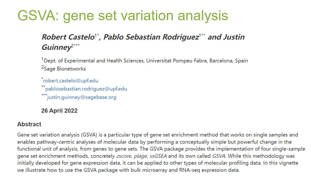
官方文档：GSVA: gene set variation analysis (bioconductor.org)不错的一篇文章：GSVA的使用 - raisok

定义基因集变异分析(GSVA)是一种特殊类型的基因集富集方法，通过对分析的功能单元进行概念上简单但功能强大的改变——从基因到基因集，从而实现对分子数据的路径中心分析。 简单来说，就是将分析对象由基因换成了基因集，进行基因集（通路）级别的差异分析。
原理和作用通过将基因在不同样品间的表达量矩阵转化成基因集在样品间的表达量矩阵，从而来评估不同的通路在不同样品间是否富集。其实就是研究这些感兴趣的基因集在不同样品间的差异，或者寻找比较重要的基因集，作为一种分析方法，主要是是为了从生物信息学的角度去解释导致表型差异的原因。

GSVA官方定义.png

分析前准备：

rm(list = ls())
options(stringsAsFactors = F)
library(tidyverse)
library(clusterProfiler)
library(msigdbr)  #install.packages("msigdbr")
library(GSVA) 
library(GSEABase)
library(pheatmap)
library(limma)
library(BiocParallel)

setwd("C:/Users/Lenovo/Desktop/test")
source('FUNCTIONS.R')
load(file = '1.counts.Rdata') #包含 tpm counts group_list gl
dir.create("6.GSVA"); setwd("6.GSVA")

复制

2.下载GSVA分析所需的基因集

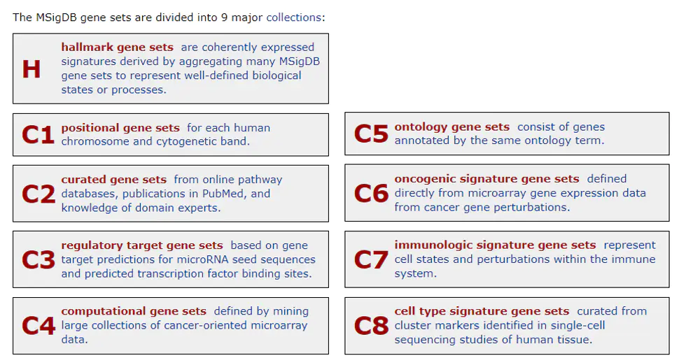
GSVA分析常用MSigDB数据库中基因集，也可以自定义基因集进行分析。 MSigDB数据库目前有H和C1-C8九个定义的基因集，下面示范下载包含KEGG信息的C2与包含GO信息的C5基因集的两种方式——手动下载读取或msigdbr包下载提取。

2.1 手动下载读取

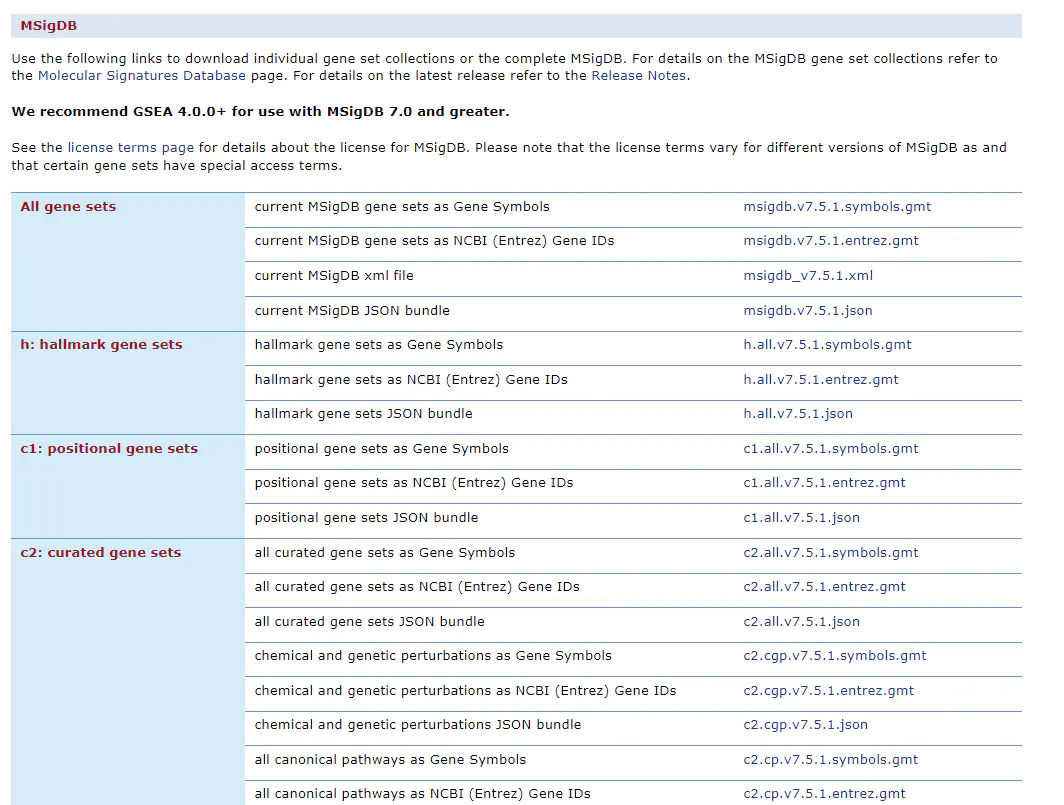
下载地址：Downloads (gsea-msigdb.org)进入gsea-msigdb官网后可能还需要登录邮箱，然后找到需要下载的基因集下载，下载后将gmt文件放入指定文件夹，将其路径读取进入R即可。不过需要注意的是这里的基因集默认都是人类的，如果是分析小鼠或其他物种最好采用MigDB包下载

#### 对 MigDB( Molecular Signatures Database)中的基因集做GSVA分析  ####
## 用手动下载基因集做GSVA分析
d <- 'C:/Users/Lenovo/Desktop/test/gmt' #存放gmt文件的路径
gmtfs <- list.files(d,pattern = 'symbols.gmt')  # 路径下所有结尾为symbols.gmt文件
gmtfs
kegg_list <- getGmt(file.path(d,gmtfs[1])) 
go_list <- getGmt(file.path(d,gmtfs[2]))

复制

2.2 msigdbr包下载读取

使用msigdbr包可以直接在R里下载C2和C5基因集，并提取相关信息做成list。 msigdbr下载数据可以指定物种，用msigdbr_species() 和 msigdbr_collections()可以查看支持的物种和基因集类别。以下参考：GSEA和GSVA，再也不用去下载gmt文件咯

## msigdbr包提取下载 一般尝试KEGG和GO做GSVA分析
##KEGG
KEGG_df_all <-  msigdbr(species = "Mus musculus", # Homo sapiens or Mus musculus
                        category = "C2",
                        subcategory = "CP:KEGG") 
KEGG_df <- dplyr::select(KEGG_df_all,gs_name,gs_exact_source,gene_symbol)
kegg_list <- split(KEGG_df$gene_symbol, KEGG_df$gs_name) ##按照gs_name给gene_symbol分组

##GO
GO_df_all <- msigdbr(species = "Mus musculus",
                     category = "C5")  
GO_df <- dplyr::select(GO_df_all, gs_name, gene_symbol, gs_exact_source, gs_subcat)
GO_df <- GO_df[GO_df$gs_subcat!="HPO",]
go_list <- split(GO_df$gene_symbol, GO_df$gs_name) ##按照gs_name给gene_symbol分组

复制

3. GSVA的运行

使用GSVA需要输入基因表达矩阵和基因集。基因集即为我们上一步所得list；基因表达矩阵可以使用logCPM、logRPKM、logTPM（GSVA参数kcdf选择"Gaussian"，默认）或counts数据（参数kcdf选择"Poisson"）。 GSVA还支持BiocParallel，可设置参数parallel.sz进行多核计算。下面选取基因集go_list和logTPM数据进行示范

####  GSVA  ####
#GSVA算法需要处理logCPM, logRPKM,logTPM数据或counts数据的矩阵####
#dat <- as.matrix(counts)
#dat <- as.matrix(log2(edgeR::cpm(counts))+1)
dat <- as.matrix(log2(tpm+1))

geneset <- go_list

gsva_mat <- gsva(expr=dat, 
               gset.idx.list=geneset, 
               kcdf="Gaussian" ,#"Gaussian" for logCPM,logRPKM,logTPM, "Poisson" for counts
               verbose=T, 
               parallel.sz = parallel::detectCores())#调用所有核

write.csv(gsva_mat,"gsva_go_matrix.csv")

复制

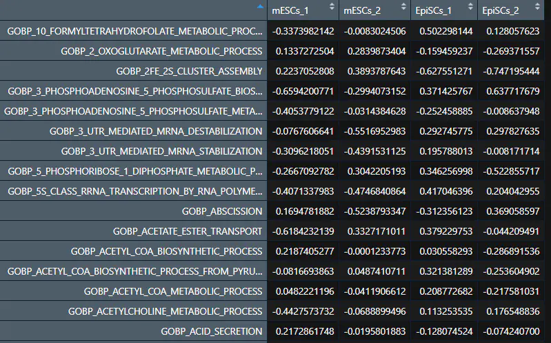
运行完GSVA后gsva_mat内容如下，可以发现行名变成了基因集通路名，每个样品都会有对应通路的GSVA评分：

4. limma差异分析

得到GSVA评分的矩阵后，我们需要利用limma包进行pathway通路的差异分析，与之前介绍的基因差异分析流程类似，但不需要进行 limma-trend 或 voom的步骤

#### 进行limma差异处理 ####
##设定 实验组exp / 对照组ctr
gl
exp="primed"
ctr="naive"

design <- model.matrix(~0+factor(group_list))
colnames(design) <- levels(factor(group_list))
rownames(design) <- colnames(gsva_mat)
contrast.matrix <- makeContrasts(contrasts=paste0(exp,'-',ctr),  #"exp/ctrl"
                                 levels = design)

fit1 <- lmFit(gsva_mat,design)                 #拟合模型
fit2 <- contrasts.fit(fit1, contrast.matrix) #统计检验
efit <- eBayes(fit2)                         #修正

summary(decideTests(efit,lfc=1, p.value=0.05)) #统计查看差异结果
tempOutput <- topTable(efit, coef=paste0(exp,'-',ctr), n=Inf)
degs <- na.omit(tempOutput) 
write.csv(degs,"gsva_go_degs.results.csv")

复制

5. GSVA结果可视化：热图、火山图、发散条形图/柱形偏差图

与常规差异分析结果展示类似，GSVA结果可视化一般也用热图、火山图展示

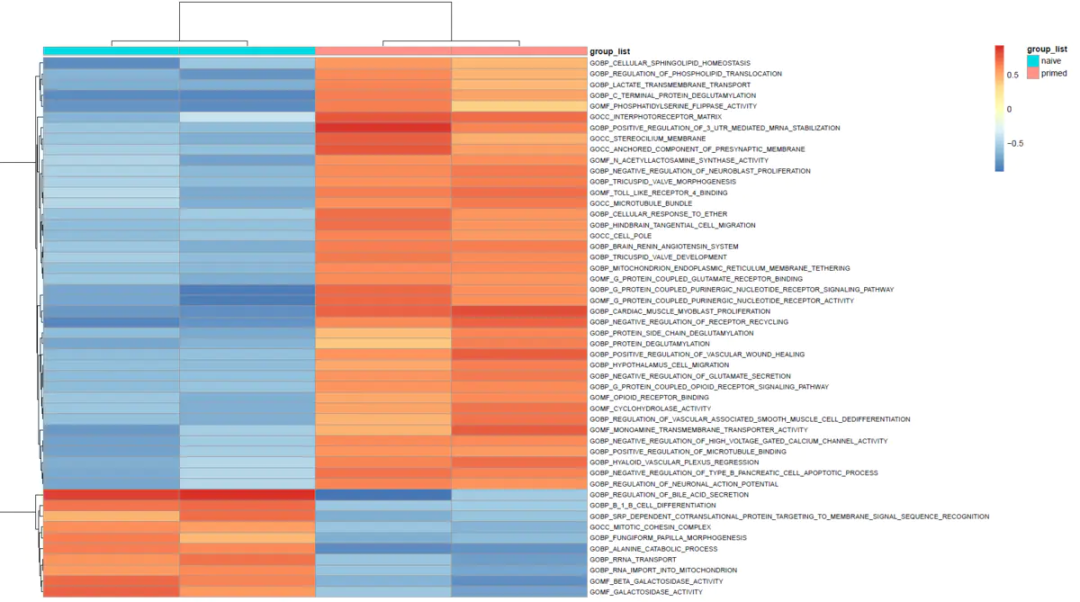
5.1 热图

#### 对GSVA的差异分析结果进行热图可视化 #### 
##设置筛选阈值
padj_cutoff=0.05
log2FC_cutoff=log2(2)

keep <- rownames(degs[degs$adj.P.Val < padj_cutoff & abs(degs$logFC)>log2FC_cutoff, ])
length(keep)
dat <- gsva_mat[keep[1:50],] #选取前50进行展示

pheatmap::pheatmap(dat, 
                   fontsize_row = 8,
                   height = 10,
                   width=18,
                   annotation_col = gl,
                   show_colnames = F,
                   show_rownames = T,
                   filename = paste0('GSVA_go_heatmap.pdf'))

复制

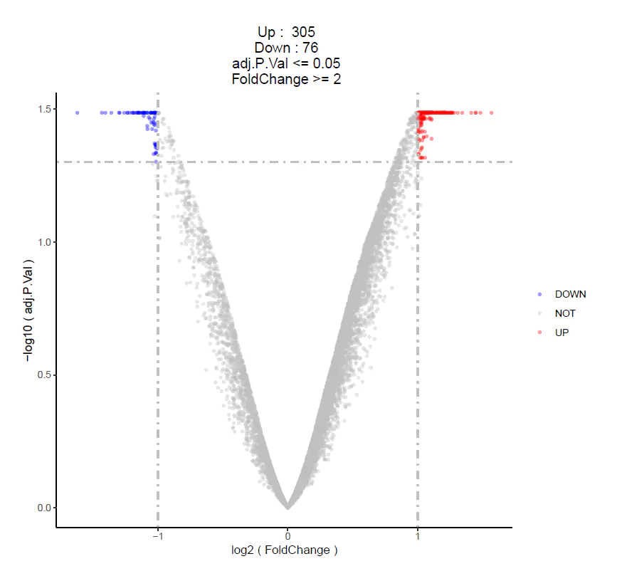
5.2 火山图

degs$significance  <- as.factor(ifelse(degs$adj.P.Val < padj_cutoff & abs(degs$logFC) > log2FC_cutoff,
                                           ifelse(degs$logFC > log2FC_cutoff ,'UP','DOWN'),'NOT'))

this_title <- paste0(' Up :  ',nrow(degs[degs$significance =='UP',]) ,
                     '\n Down : ',nrow(degs[degs$significance =='DOWN',]),
                     '\n adj.P.Val <= ',padj_cutoff,
                     '\n FoldChange >= ',round(2^log2FC_cutoff,3))


g <- ggplot(data=degs, 
            aes(x=logFC, y=-log10(adj.P.Val),
                color=significance)) +
  #点和背景
  geom_point(alpha=0.4, size=1) +
  theme_classic()+ #无网格线
  #坐标轴
  xlab("log2 ( FoldChange )") + 
  ylab("-log10 ( adj.P.Val )") +
  #标题文本
  ggtitle( this_title ) +
  #分区颜色                   
  scale_colour_manual(values = c('blue','grey','red'))+ 
  #辅助线
  geom_vline(xintercept = c(-log2FC_cutoff,log2FC_cutoff),lty=4,col="grey",lwd=0.8) +
  geom_hline(yintercept = -log10(padj_cutoff),lty=4,col="grey",lwd=0.8) +
  #图例标题间距等设置
  theme(plot.title = element_text(hjust = 0.5), 
        plot.margin=unit(c(2,2,2,2),'lines'), #上右下左
        legend.title = element_blank(),
        legend.position="right")

ggsave(g,filename = 'GSVA_go_volcano_padj.pdf',width =8,height =7.5)

复制

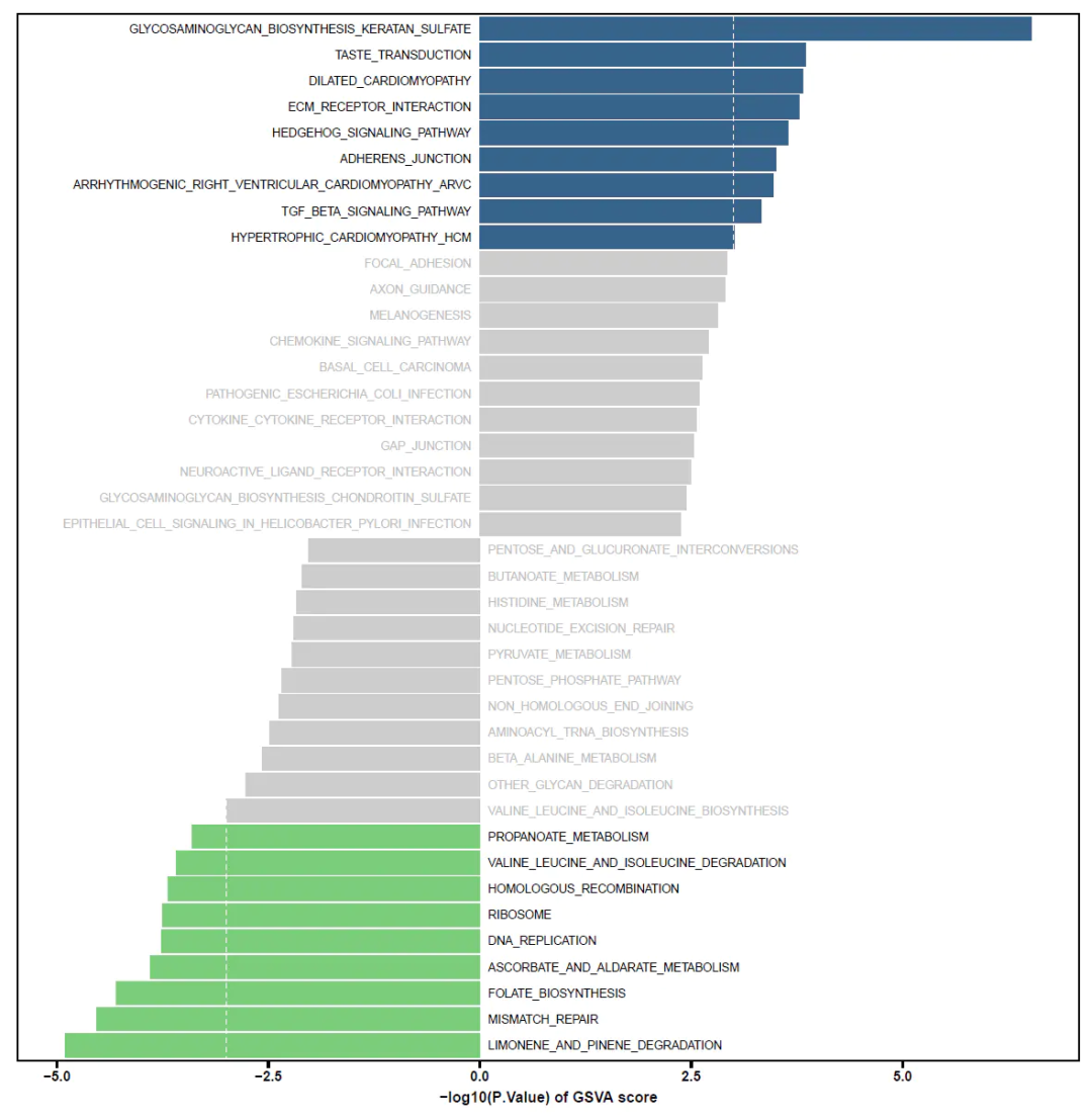
5.3 发散条形图/柱形偏差图

为了更好展示绘制发散条形图/柱形偏差图，此处用的是KEGG的gsva差异分析结果，展示通路的上下调及pvalue信息（也可以是t值或padj值等），详细绘图过程见发散条形图/柱形偏差图 - 简书 (jianshu.com)

#### 发散条形图绘制 ####
library(tidyverse)  # ggplot2 stringer dplyr tidyr readr purrr  tibble forcats
library(ggthemes)
library(ggprism)
p_cutoff=0.001
degs <- gsva_kegg_degs  #载入gsva的差异分析结果
Diff <- rbind(subset(degs,logFC>0)[1:20,], subset(degs,logFC<0)[1:20,]) #选择上下调前20通路     
dat_plot <- data.frame(id  = row.names(Diff),
                       p   = Diff$P.Value,
                       lgfc= Diff$logFC)
dat_plot$group <- ifelse(dat_plot$lgfc>0 ,1,-1)    # 将上调设为组1，下调设为组-1
dat_plot$lg_p <- -log10(dat_plot$p)*dat_plot$group # 将上调-log10p设置为正，下调-log10p设置为负
dat_plot$id <- str_replace(dat_plot$id, "KEGG_","");dat_plot$id[1:10]
dat_plot$threshold <- factor(ifelse(abs(dat_plot$p) <= p_cutoff,
                                   ifelse(dat_plot$lgfc >0 ,'Up','Down'),'Not'),
                            levels=c('Up','Down','Not'))

dat_plot <- dat_plot %>% arrange(lg_p)
dat_plot$id <- factor(dat_plot$id,levels = dat_plot$id)

## 设置不同标签数量
low1 <- dat_plot %>% filter(lg_p < log10(p_cutoff)) %>% nrow()
low0 <- dat_plot %>% filter(lg_p < 0) %>% nrow()
high0 <- dat_plot %>% filter(lg_p < -log10(p_cutoff)) %>% nrow()
high1 <- nrow(dat_plot)

p <- ggplot(data = dat_plot,aes(x = id, y = lg_p, 
                                fill = threshold)) +
  geom_col()+
  coord_flip() + 
  scale_fill_manual(values = c('Up'= '#36638a','Not'='#cccccc','Down'='#7bcd7b')) +
  geom_hline(yintercept = c(-log10(p_cutoff),log10(p_cutoff)),color = 'white',size = 0.5,lty='dashed') +
  xlab('') + 
  ylab('-log10(P.Value) of GSVA score') + 
guides(fill="none")+
  theme_prism(border = T) +
  theme(
    axis.text.y = element_blank(),
    axis.ticks.y = element_blank()
  ) +
  geom_text(data = dat_plot[1:low1,],aes(x = id,y = 0.1,label = id),
              hjust = 0,color = 'black') + #黑色标签
  geom_text(data = dat_plot[(low1 +1):low0,],aes(x = id,y = 0.1,label = id),
            hjust = 0,color = 'grey') + # 灰色标签
  geom_text(data = dat_plot[(low0 + 1):high0,],aes(x = id,y = -0.1,label = id),
            hjust = 1,color = 'grey') + # 灰色标签
  geom_text(data = dat_plot[(high0 +1):high1,],aes(x = id,y = -0.1,label = id),
            hjust = 1,color = 'black') # 黑色标签

ggsave("GSVA_barplot_pvalue.pdf",p,width = 15,height  = 15)

复制