


该推文首发于公众号:单细胞天地
在完成了马拉松课程后,我们应该对单细胞分析有了基本了解。接下来,我们将开启新的篇章——单细胞实战:从入门到进阶。
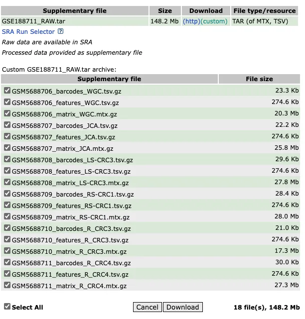
我们采用的示例数据集来自GSE188711,该数据集一共包含了6个单细胞测序样本(其中包含了3个左边结肠和3个右半结肠的样本),并采用Illumina NovaSeq 6000平台完成测序。首先我们需要从GEO官网中下载该数据集。今后很长一段时间,我们将围绕这个数据集展开一系列的分析学习。
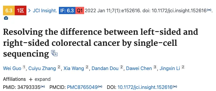
对应的文献是2022年1月发表在JCI insight上的Resolving the difference between left-sided and right-sided colorectal cancer by single-cell sequencing. PMID:34793335.
此外,可以通过向公众号发送关键词‘单细胞’,直接获取Seurat V5版本的完整代码。

本次推文中,我们将重点复习并学习降维聚类过程中的三个重要步骤:样本整理,细胞注释和部分图表绘制。
分析步骤
1.整理数据
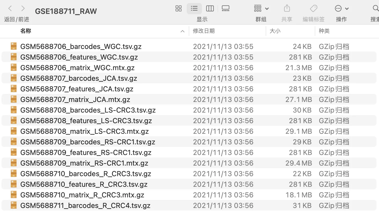
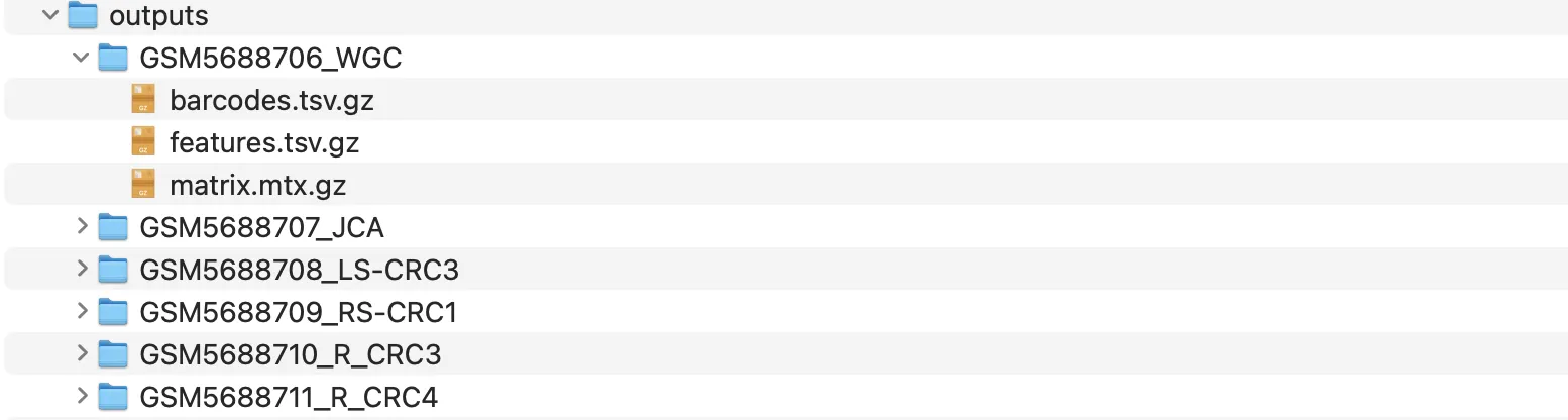
下载完数据之后,我们需要考虑怎么把数据进行归类整理。这种类型的数据需要把同一样本中的barcodes,features和matrix归类到一个文件夹中,并在最终归类的文件夹中的文件只需要保留barcodes,features和matrix名称。同时我们也需要考虑到为了更好区分不同样本的信息,默认的文件名称是GSM编号和样本信息,如果样本数量很少,比如这里一共就6个样本,那么手动分组其实也未尝不可。
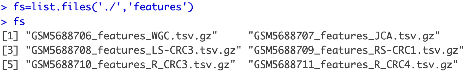
fs=list.files('./','features')
fs
samples1 = fs
samples2=gsub('_features','',fs)
samples2
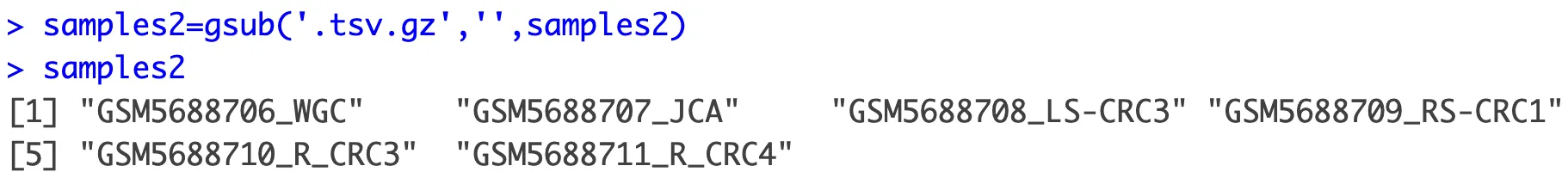
samples2=gsub('.tsv.gz','',samples2)
samples2
# 创建 outputs 文件夹
dir.create("outputs", showWarnings = FALSE)
lapply(1:length(samples2), function(i){
#i=1
x=samples2[i]
y=samples1[i]
x;y
# 创建子目录路径
output_dir = file.path("outputs", x)
dir.create(output_dir, recursive = TRUE)
# 移动并重命名文件
file.copy(from = y,
to = file.path(output_dir, 'features.tsv.gz'))
file.copy(from = gsub('tsv', 'mtx', gsub('features', 'matrix', y)),
to = file.path(output_dir, 'matrix.mtx.gz'))
file.copy(from = gsub('features', 'barcodes', y),
to = file.path(output_dir, 'barcodes.tsv.gz'))
})
这段代码我们首先提取了含有features的文件名称,做这一步就是为后面进行样本和文件夹重命名做准备,同理这里用matrix,barcodes提取数据也是可以的。
得到了fs名称之后,我们需要对其进行优化,分步去除“_features”和“.tsv.gz”,最终得到了含有GSM编号和样本特征的名称,这个也将最终变成文件夹名称。
接着我们创建outputs文件夹用于保存所有整合好的文件,同时我们也需要创建更新后的子目录。移动并重名文件夹的时候使用了gsub做了多次变化,并使用file.copy对文件进行了重命名。最终得到如下的文件夹+文件。
2.降维聚类分群
使用Seurat V5
rm(list=ls())
options(stringsAsFactors = F)
source('scRNA_scripts/lib.R')
getwd()
step1:导入数据
###### step1: 导入数据 ######
# 付费环节 800 元人民币
# 参考:https://mp.weixin.qq.com/s/tw7lygmGDAbpzMTx57VvFw
dir='/Users/zaneflying/Desktop/practiceGSE188711/GSE188711_RAW/outputs/'
samples=list.files(dir)
samples
library(data.table)
sceList = lapply(samples,function(pro){
sce = CreateSeuratObject(counts =  Read10X(file.path(dir,pro)) ,
                         project = pro,
                         min.cells = 5,
                         min.features = 300 )
return(sce)
})
# 把scrList的每个样本进行命名
names(sceList) =  samples
# 合并样本
sce.all <- merge(sceList[[1]], y= sceList[ -1 ] ,
                 add.cell.ids =  samples)
dim(sce.all)
# [1] 21308 32300
# V5版本的需要joinLayers
LayerData(sce.all, assay = "RNA", layer = "counts")
sce.all <- JoinLayers(sce.all)
dim(sce.all[["RNA"]]$counts )
sp='human'
step2:QC质控
# 如果为了控制代码复杂度和行数
# 可以省略了质量控制环节
###### step2: QC质控 ######
dir.create("./1-QC")
setwd("./1-QC")
# 如果过滤的太狠,就需要去修改这个过滤代码
source('../scRNA_scripts/qc.R')
sce.all.filt = basic_qc(sce.all)
print(dim(sce.all))
#[1] 21308 32300
print(dim(sce.all.filt))
#[1] 21308 25621
setwd('../')
getwd()
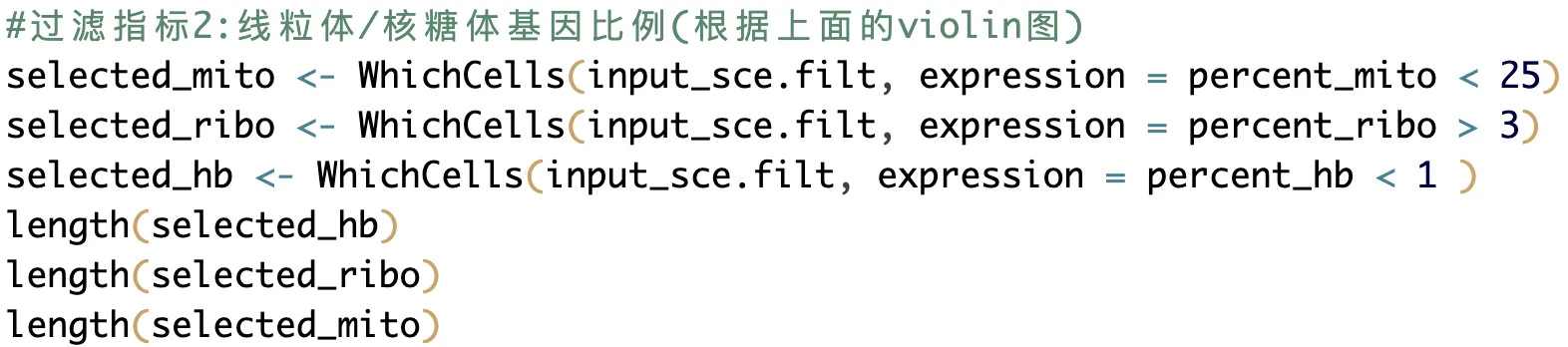
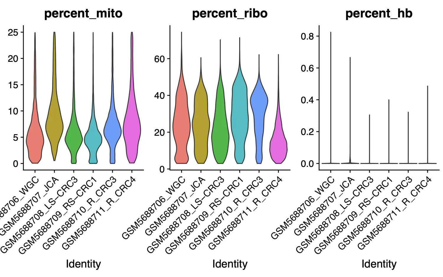
QC中设定了筛选线粒体基因百分比小于 25% ,核糖体基因表达比例大于 3%和血红蛋白基因表达比例小于 1%的细胞,关于过滤标准需要按照不同组织进行划分,目前没有“确定”的标准。原文质控完之后的细胞数目为27927,我们这里的细胞数据为25621,数量上是有差别的,但这也是无法避免的,通常很难做到得到跟原作者一样的数据结果。
step3:harmony整合多个单细胞样品
###### step3: harmony整合多个单细胞样品 ######
if(T){
  dir.create("2-harmony")
  getwd()
  setwd("2-harmony")
  source('../scRNA_scripts/harmony.R')
  # 默认 ScaleData 没有添加"nCount_RNA", "nFeature_RNA"
  # 默认的
  sce.all.int = run_harmony(sce.all.filt)
  setwd('../')
}
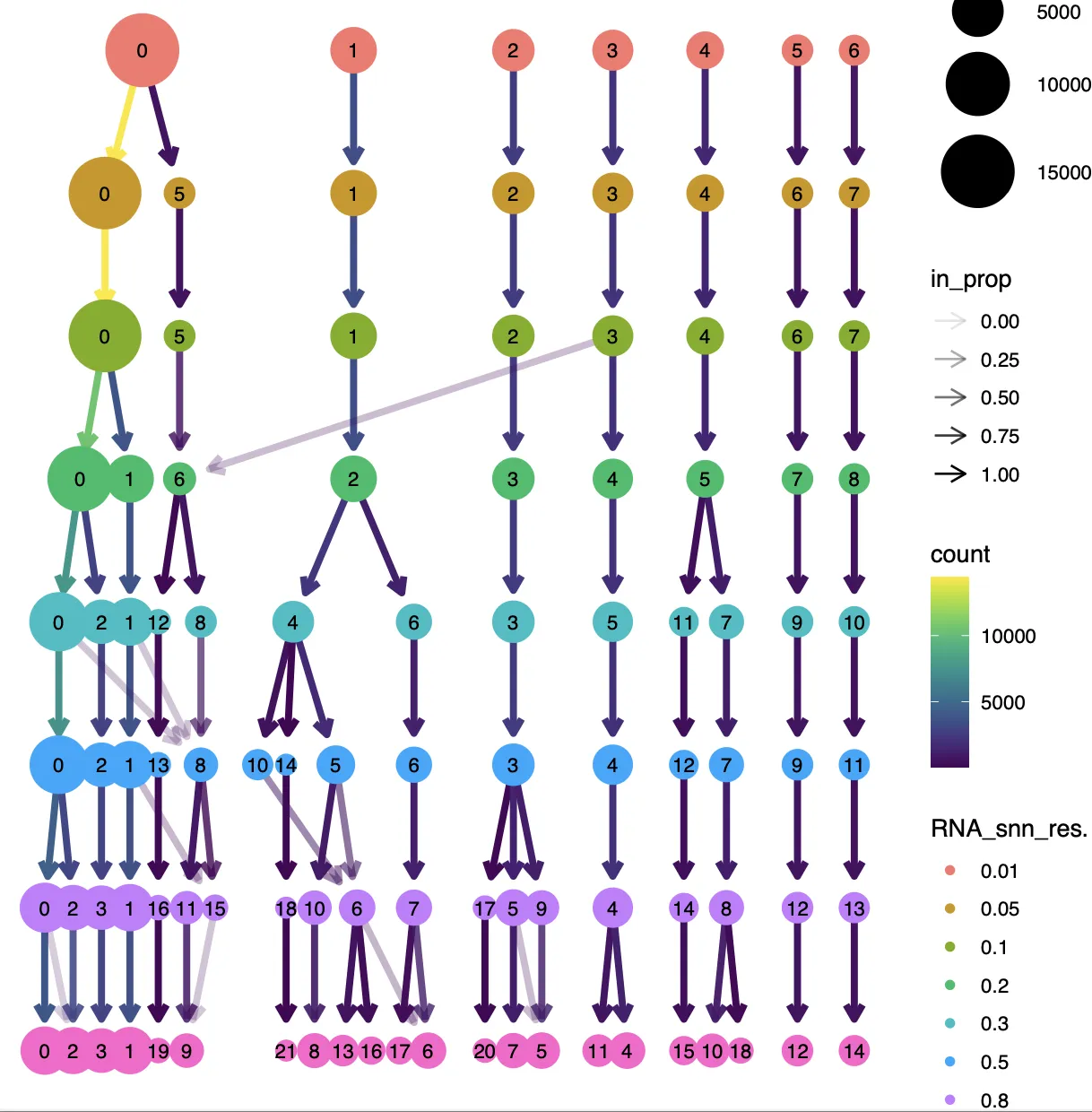
原文中分辨率选择了0.6,而根据进化树和分群情况情况,可以有两种策略,第一种是选择较低的分辨率(比如0.2)进行粗分,之后再进行细分,第二种是选择较高的分辨率(比如0.8)粗分之后再进行修整。两种方法都可以,也都需要经过粗分到细分过程。本次分辨率选择0.8进行分群。
step4:看标记基因库
###### step4:  看标记基因库 ######
table(Idents(sce.all.int))
table(sce.all.int$seurat_clusters)
table(sce.all.int$RNA_snn_res.0.1)
table(sce.all.int$RNA_snn_res.0.8)

getwd()
dir.create('check-by-0.1')
setwd('check-by-0.1')
sel.clust = "RNA_snn_res.0.1"
sce.all.int <- SetIdent(sce.all.int, value = sel.clust)
table(sce.all.int@active.ident)

source('../scRNA_scripts/check-all-markers.R')
setwd('../')
getwd()

dir.create('check-by-0.5')
setwd('check-by-0.5')
sel.clust = "RNA_snn_res.0.5"
sce.all.int <- SetIdent(sce.all.int, value = sel.clust)
table(sce.all.int@active.ident)
source('../scRNA_scripts/check-all-markers.R')
setwd('../')
getwd()

dir.create('check-by-0.8')
setwd('check-by-0.8')
sel.clust = "RNA_snn_res.0.8"
sce.all.int <- SetIdent(sce.all.int, value = sel.clust)
table(sce.all.int@active.ident)
source('../scRNA_scripts/check-all-markers.R')
setwd('../')
getwd()

last_markers_to_check
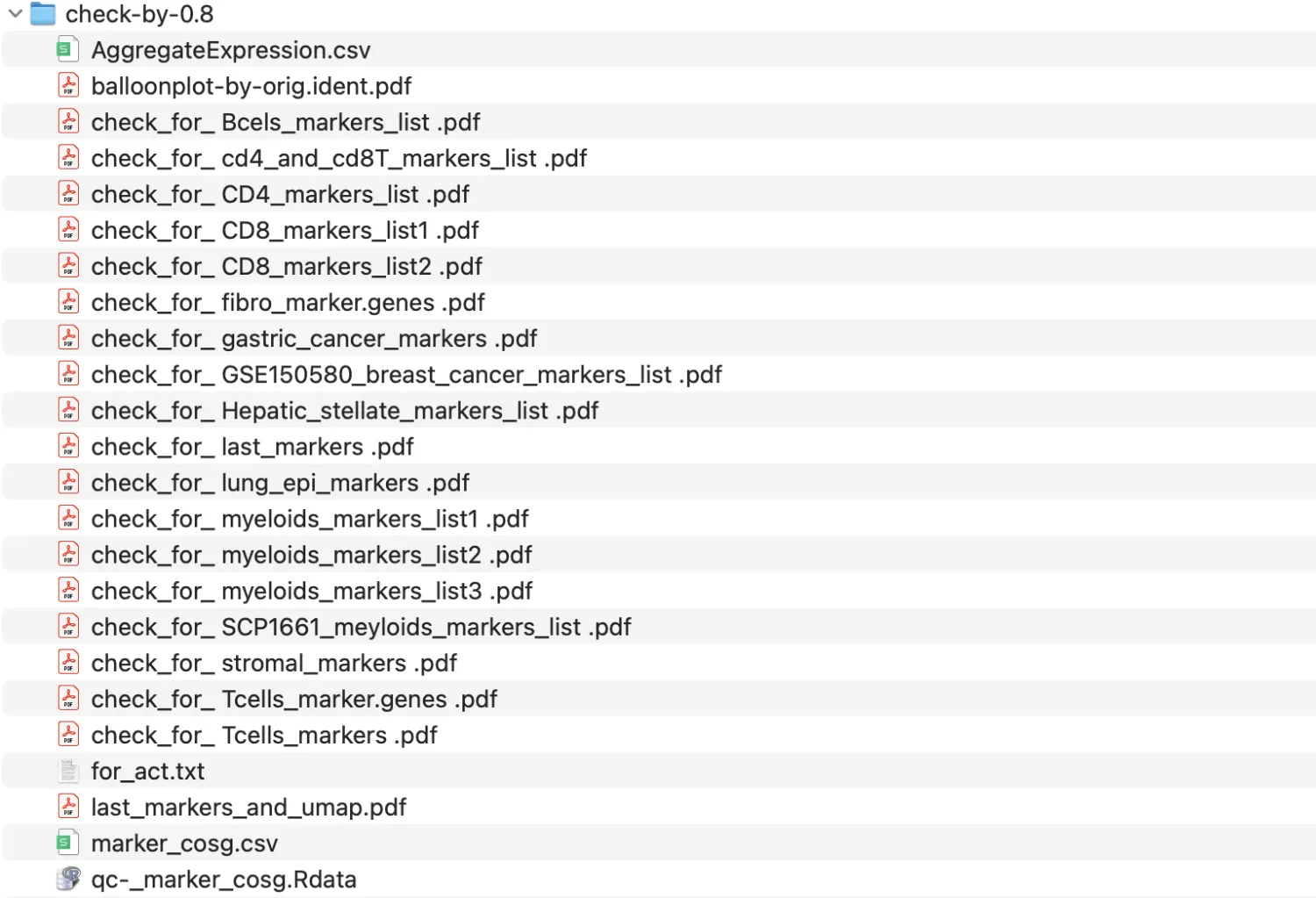
曾老师的代码中包含了多种细胞和肿瘤的标记库,此外还存在COSG函数分析得到了每个细胞群中的差异基因。 接下来重点查看0.8分辨率的结果,笔者查看标记结果的方法主要为以下12个字:由浅入深,重点关注,反复对比。
查看结果的具体顺序为1. Last_markers_and_umap结果;2.查看需要特别关注或者last_markers_and_umap结果中不明确或者特定组织特定标记群结果;3.查看对比cosg/findallmarkers等差异基因分析工具得到的结果,时刻提醒自己要结合生物学知识。
-
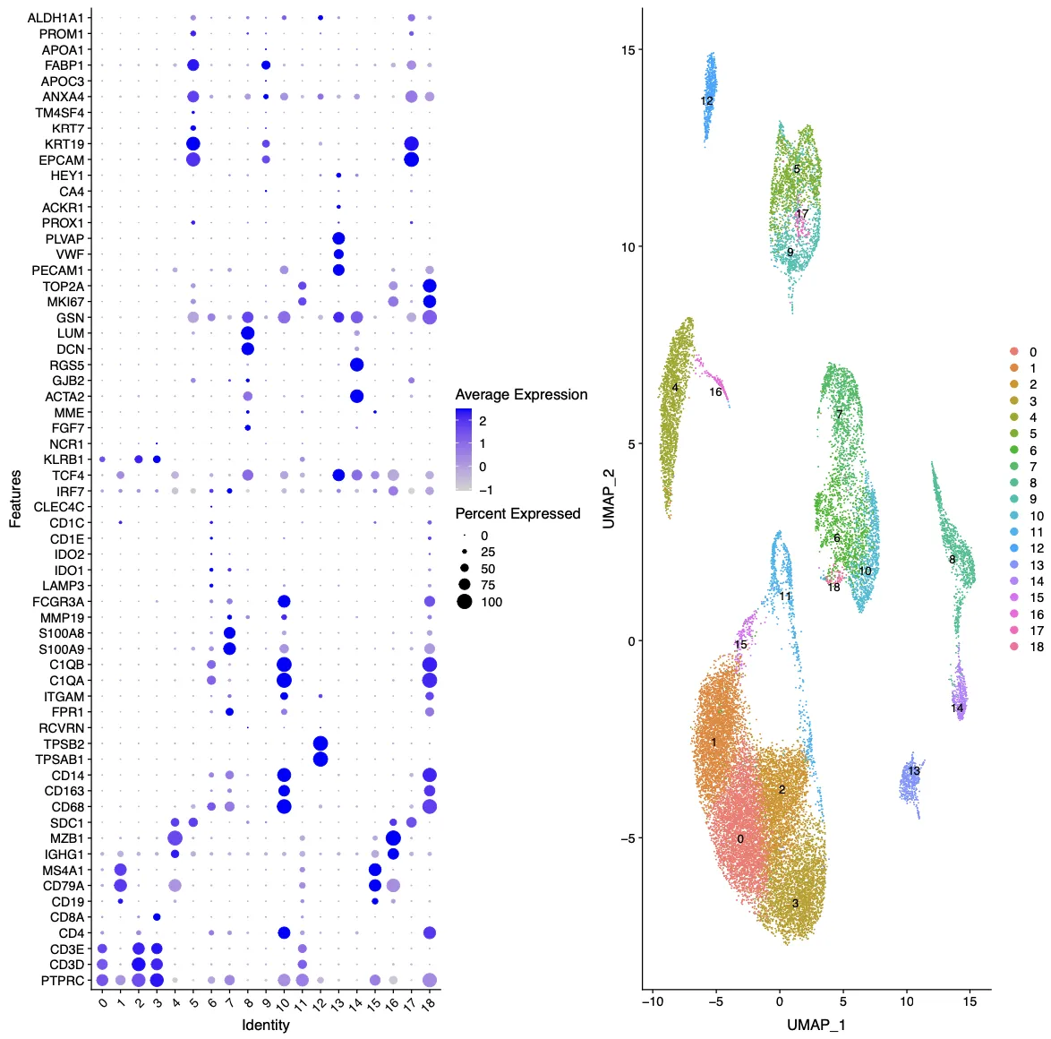
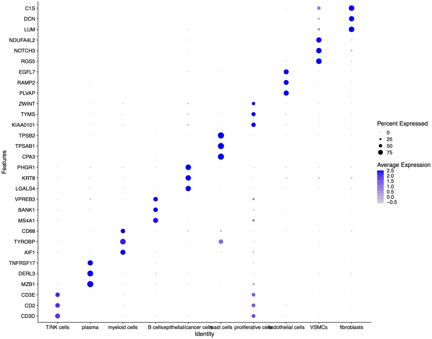
Last_markers_and_umap的结果是气泡图结合UMAP图:这里的标记主要是目前我们所已知公认的标记,每个人都可以根据自己主攻方向设定标记集。除此之外,我们也需要根据UMAP图中的不同细胞群之间的位置和细胞群的信息来反推我们的注释是否存在问题。
-
查看需要特别关注或者last_markers_and_umap结果中不明确或者特定组织特定标记群结果。比如在后续分析中需要特别关注T细胞,那么可以尝试先观察一下T细胞标记集的结果;或者比如在last_markers_and_umap结果中发现某一群细胞无法被清晰的注释,那么就可以考虑通过更加细节的标记进一步对比
-
查看对比cosg/findallmarkers等差异基因分析工具得到的结果,时刻提醒自己要结合生物学知识。根据差异分析基因工具得到不同细胞群中的差异基因,然后根据这些差异基因去验证前面两步注释的结果。
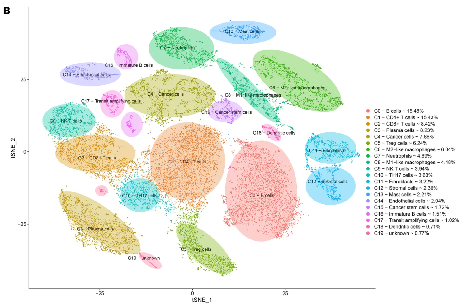
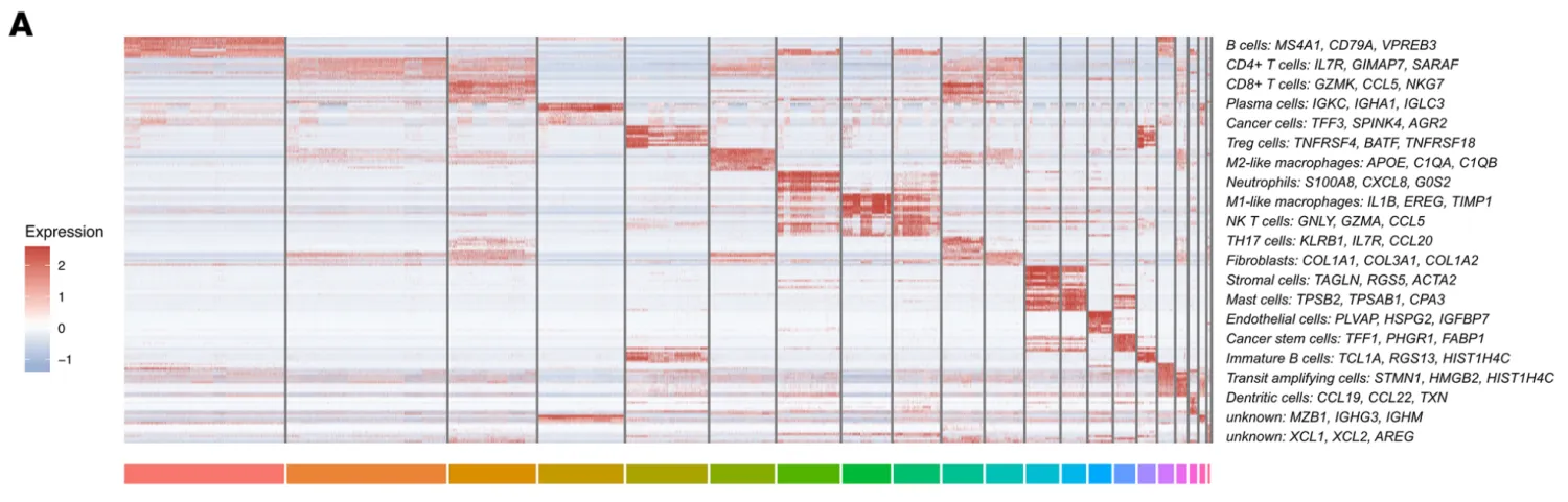
接下来打算正式对细胞进行注释分群,首先回溯一下文章中的分群情况以及每个细胞群所对应的标志物。研究者将细胞十分细致的分成了19个亚群,特别有意思的是研究者还分出了一群Cancer stem cells细胞群,这群细胞的高表达标记物为TFF3, SPKK4, AGR2。不过按照目前的研究来看,可能还需要更多的标志物才能更好的定义干细胞。
作为一个示例数据,我们并不计划严格按照研究者提供的细胞分群信息进行细胞注释,而是结合以下信息综合进行细胞注释。
-
细胞亚群的认定流程:第一:判断标志物是否是细胞群所特有的,比如T细胞的CD3, B细胞的MS4A1(CD20),NK细胞的KLRB1,髓系细胞的C1QA/C1QB,肝细胞的APOC3。第二:需要考虑标志物的平均表达量高低,一般会倾向关注表达量很高的标志物。第三:若两种分属不同细胞亚群的标志物在同一个细胞簇中出现时,需要考虑是否是特殊的细胞群。
-
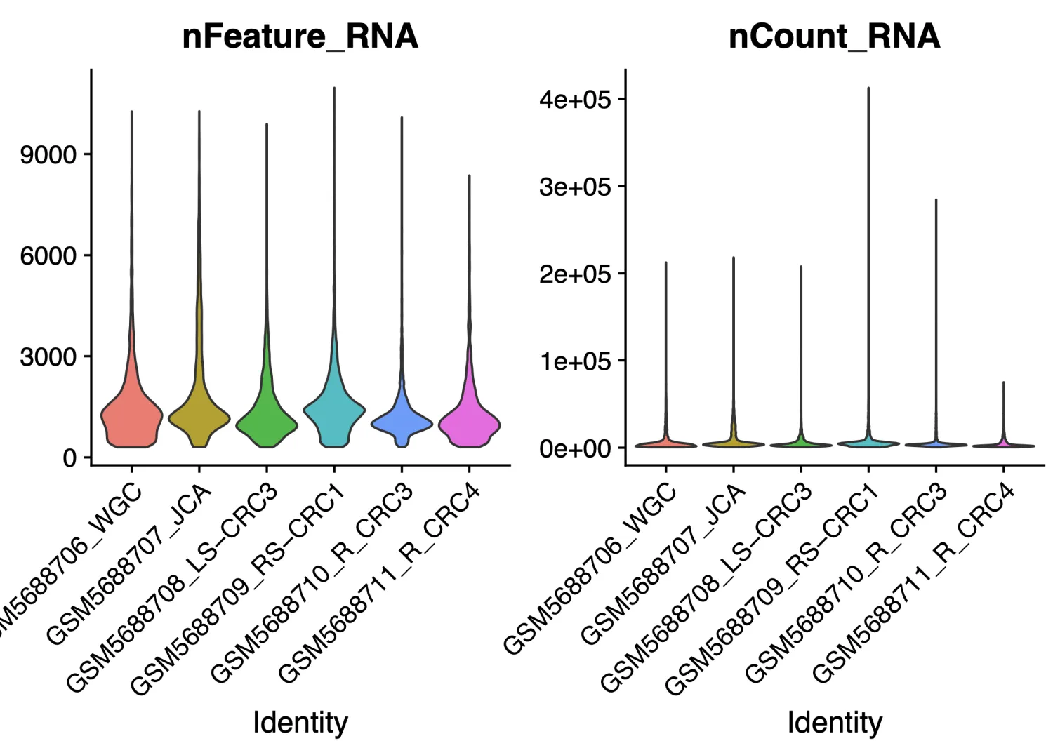
如果细胞群出现特殊情况,举个不恰当的例子,比如在下面这个图中有那么多个簇都属于T细胞的时候,需要考虑是否是存在问题(要考虑T细胞的数量和百分比是否符合常理),这个时候需要回溯多个图表进行综合考量。比如需要回溯nFeature,nCount图看看这个簇的值是否异常(包括线粒体,核糖体和血红蛋白的值),也需要看看COSG/FindAllmaker差异分析结果判断一下是否符合T细胞的特征,同时一定要查阅一下文献看看是否有高分文献进行过类型细胞的报道。如果确认了上述情况都没有问题,那咱们也不要犹豫,这就是真实的结果~ 后续就可以继续研究为什么这批样本中T细胞的比例如此之高。
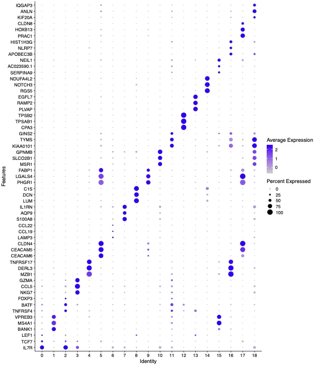
cosg结果与前面的结果对比验证
step5: 确定单细胞亚群生物学名字
###### step5: 确定单细胞亚群生物学名字 ######
source('scRNA_scripts/lib.R')
sce.all.int = readRDS('2-harmony/sce.all_int.rds')
sp='human'
tmp=sce.all.int@meta.data
colnames(sce.all.int@meta.data)
table(sce.all.int$RNA_snn_res.0.8)
# pbmc_small <- BuildClusterTree(object = sce.all.int)
# plot(Tool(object = pbmc_small, slot = 'BuildClusterTree'))
# plot(pbmc_small@tools$BuildClusterTree)

# 付费环节 800 元人民币
# 如果是手动给各个单细胞亚群命名
if(T){
  sce.all.int
  celltype=data.frame(ClusterID=0:18 ,
                      celltype= 0:18  )
  #定义细胞亚群
  celltype[celltype$ClusterID %in% c( 0,2,3  ),2]='T/NK cells'
  celltype[celltype$ClusterID %in% c( 1,15  ),2]='B cells'
  celltype[celltype$ClusterID %in% c( 4,16  ),2]='plasma'
  celltype[celltype$ClusterID %in% c( 11  ),2]='proliferative cells'
  celltype[celltype$ClusterID %in% c( 10,18  ),2]='macrophages'
  celltype[celltype$ClusterID %in% c( 7  ),2]='neutrophils'
  celltype[celltype$ClusterID %in% c( 13  ),2]='endothelial cells'
  celltype[celltype$ClusterID %in% c( 8 ),2]='fibroblasts'
  celltype[celltype$ClusterID %in% c( 5,9,17 ),2]='epithelial/cancer cells'
  celltype[celltype$ClusterID %in% c( 12 ),2]='mast cells'
  celltype[celltype$ClusterID %in% c( 14 ),2]='VSMCs'
  celltype[celltype$ClusterID %in% c( 6 ),2]='dendritic cells'
  sce.all.int
  head(celltype)
  celltype
  table(celltype$celltype)
  sce.all.int@meta.data$celltype = "NA"

  for(i in 1:nrow(celltype)){
    sce.all.int@meta.data[which(sce.all.int@meta.data$RNA_snn_res.0.8 == celltype$ClusterID[i]),'celltype'] <- celltype$celltype[i]}
  Idents(sce.all.int)=sce.all.int$celltype


}

table(sce.all.int$celltype)
# B cells         dendritic cells       endothelial cells epithelial/cancer cells
# 3804                    1244                     549                    2421
# fibroblasts             macrophages              mast cells             neutrophils
# 1040                    1014                     596                    1198
# plasma     proliferative cells              T/NK cells                   VSMCs
# 2096                     803                   10445                     411
在这一次分群中,一共分出了12种细胞,分别为B cells,dendritic cells,endothelial cells,epithelial/cancer cells, fibroblasts,macrophages,mast cells,neutrophils,plasma,proliferative cells,T/NK cells,VSMCs。
接下来我们可以先大概粗看一下每个细胞亚群的细胞数量,其中dendritic cells, macrophages和neutrophils这几个群数据过于相近!而根据我们的先验知识,通常树突细胞在免疫细胞中占比是最少的,中性粒细胞比例会高一些,巨噬细胞在这三种细胞中占比是最高的。因此在看到三者的细胞数量过于相似时需要警惕这种注释方式是否正确。
那么回溯的注释是否正确的顺序可以从以下几点考虑:1. 首先是回看标志物的气泡图和UMAP图;2.如果确定无误,那么就要从样本的生物学角度考虑是否符合“逻辑”;3.如果都是正确的那就大胆的命名,如果拿不准那就退一步往这些细胞群的上一级命名。 那么根据这几点回溯了数据之后发现暂时不能确定这就是准确的细胞分群,因此我们决定将这几群细胞统一命名为myeloid cells.
# 重新注释,不需要的细胞亚群用#注释掉了
if(T){
  sce.all.int
  celltype=data.frame(ClusterID=0:18 ,
                      celltype= 0:18  )
  #定义细胞亚群
  celltype[celltype$ClusterID %in% c( 0,2,3  ),2]='T/NK cells'
  celltype[celltype$ClusterID %in% c( 1,15  ),2]='B cells'
  celltype[celltype$ClusterID %in% c( 4,16  ),2]='plasma'
  celltype[celltype$ClusterID %in% c( 11  ),2]='proliferative cells'
  #celltype[celltype$ClusterID %in% c( 10,18  ),2]='macrophages'
  #celltype[celltype$ClusterID %in% c( 7  ),2]='neutrophils'
  celltype[celltype$ClusterID %in% c( 13  ),2]='endothelial cells'
  celltype[celltype$ClusterID %in% c( 8 ),2]='fibroblasts'
  celltype[celltype$ClusterID %in% c( 5,9,17 ),2]='epithelial/cancer cells'
  celltype[celltype$ClusterID %in% c( 12 ),2]='mast cells'
  celltype[celltype$ClusterID %in% c( 14 ),2]='VSMCs'
  #celltype[celltype$ClusterID %in% c( 6 ),2]='dendritic cells'
  celltype[celltype$ClusterID %in% c( 6,7,10,18 ),2]='myeloid cells'
  sce.all.int
  head(celltype)
  celltype
  table(celltype$celltype)
  sce.all.int@meta.data$celltype = "NA"

  for(i in 1:nrow(celltype)){
    sce.all.int@meta.data[which(sce.all.int@meta.data$RNA_snn_res.0.8 == celltype$ClusterID[i]),'celltype'] <- celltype$celltype[i]}
  Idents(sce.all.int)=sce.all.int$celltype


}

table(sce.all.int$celltype)
# B cells       endothelial cells epithelial/cancer cells             fibroblasts
# 3804                     549                    2421                    1040
# mast cells           myeloid cells             plasma        proliferative cells
# 596                    3456                    2096                     803
# T/NK cells               VSMCs
# 10445                     411
我们可以看到此时三种细胞已经整合成myeloid cells了
# 过滤无法命名的
sce.all.int = sce.all.int[,!sce.all.int$celltype %in% 0:100]
table(sce.all.int$celltype)
table(sce.all.int$orig.ident)
# GSM5688706_WGC     GSM5688707_JCA GSM5688708_LS-CRC3 GSM5688709_RS-CRC1  GSM5688710_R_CRC3
# 3640               2894               5796               5354               3831
# GSM5688711_R_CRC4
# 4106
sce.all.int
# An object of class Seurat
# 21308 features across 25621 samples within 1 assay
# Active assay: RNA (21308 features, 2000 variable features)
# 3 layers present: counts, data, scale.data
# 3 dimensional reductions calculated: pca, harmony, umap
head(colnames(sce.all.int))
# [1] "GSM5688706_WGC_AAACCCAAGGCATGGT-1" "GSM5688706_WGC_AAACCCATCCGTGGGT-1"
# [3] "GSM5688706_WGC_AAACGAAAGGGCTGAT-1" "GSM5688706_WGC_AAACGAAAGGTACATA-1"
# [5] "GSM5688706_WGC_AAACGAAAGTCACGCC-1" "GSM5688706_WGC_AAACGAACAACATCGT-1"
接下来把左右半结肠的临床信息添加进去, 请至GEO官网进行查看。
a <- sce.all.int@meta.data
a$location <- ifelse(a$orig.ident %in% c("GSM5688706_WGC","GSM5688707_JCA","GSM5688708_LS-CRC3"),"left","right")
table(a$location)
# left right
# 12330 13291
sce.all.int@meta.data <- a
colnames(sce.all.int@meta.data)
# [1] "orig.ident" "nCount_RNA" "nFeature_RNA" "percent_mito" "percent_ribo" "percent_hb"
# [7] "RNA_snn_res.0.01" "seurat_clusters" "RNA_snn_res.0.05" "RNA_snn_res.0.1" "RNA_snn_res.0.2" "RNA_snn_res.0.3"
# [13] "RNA_snn_res.0.5" "RNA_snn_res.0.8" "RNA_snn_res.1" "celltype" "location"
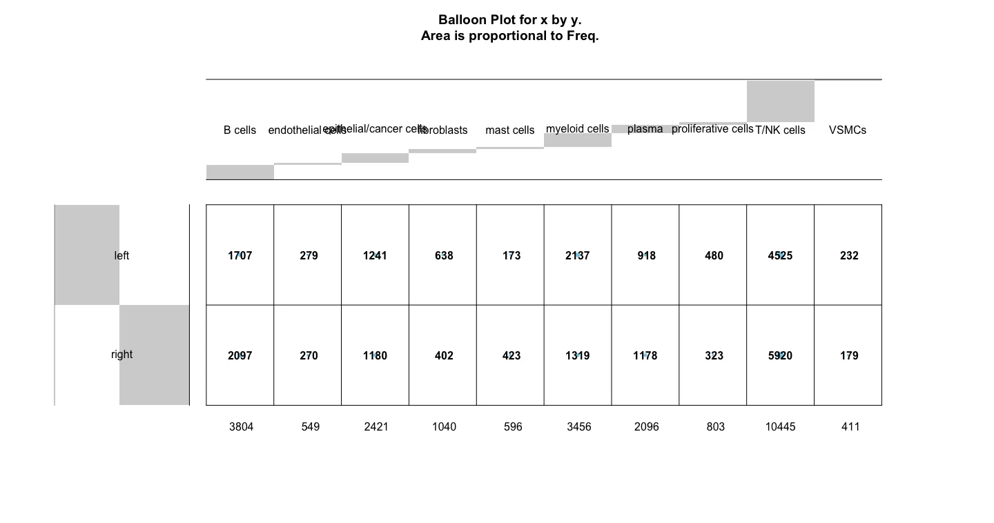
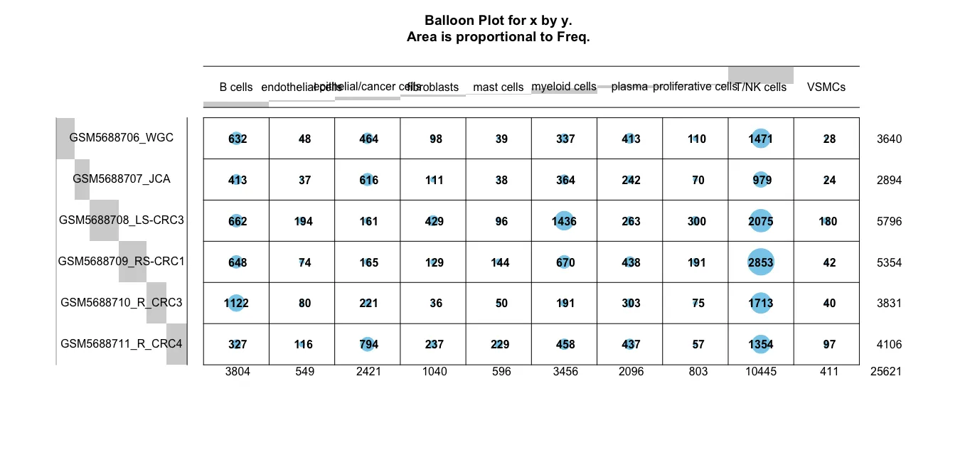
gplots::balloonplot(table(sce.all.int$celltype ,
sce.all.int$location))
gplots::balloonplot(table(sce.all.int$celltype ,
sce.all.int$orig.ident))
并通过气泡图查看一下左右半结肠中各个细胞亚群的细胞数量是否有差异。粗看下来可能mast cell在数量上是最显著的细胞群,同时对比原文中的结果发现mast细胞的比例也确实在右边结肠中比例高。
# 如果前面成功的给各个细胞亚群命名了
# 就可以运行下面的代码
if("celltype" %in% colnames(sce.all.int@meta.data ) ){

  sel.clust = "celltype"
  sce.all.int <- SetIdent(sce.all.int, value = sel.clust)
  table(sce.all.int@active.ident)
  phe=sce.all.int@meta.data
  save(phe,file = 'phe.Rdata')
  pdf('celltype-vs-orig.ident.pdf',width = 10)
  gplots::balloonplot(table(sce.all.int$celltype,sce.all.int$orig.ident))
  dev.off()

  dir.create('check-by-celltype')
  setwd('check-by-celltype')
  source('../scRNA_scripts/check-all-markers.R')
  setwd('../')
  getwd()
}
step6. 载入并且理解数据
rm(list=ls())
options(stringsAsFactors = F)
V5_path = "/Library/Frameworks/R.framework/Versions/4.4-arm64/Resources/seurat5/"
.libPaths(V5_path)
.libPaths()
library(Seurat)
library(ggplot2)
library(clustree)
library(cowplot)
library(dplyr)
library(stringr)
library(ggsci)
library(patchwork)
library(ggsci)
library(ggpubr)
library(RColorBrewer)
getwd()
dir.create('paper-figures/')
setwd('paper-figures/')
## 1. 载入,并且理解数据 ----
sce.all = readRDS('../2-harmony/sce.all_int.rds')
sp='human'
load('../phe.Rdata')
identical(rownames(phe) , colnames(sce.all))
sce.all=sce.all[,colnames(sce.all) %in% rownames(phe) ]
sce.all@meta.data = phe[match(colnames(sce.all),rownames(phe) ),]
sel.clust = "celltype"
sce.all <- SetIdent(sce.all, value = sel.clust)
table(sce.all@active.ident)
DimPlot(sce.all)
colnames(sce.all@meta.data)
sce.all.int=sce.all
seuratObj <- RunUMAP(sce.all.int,
reduction = "pca",
dims = 1:15 )
colnames(sce.all.int@meta.data)
p3=DimPlot(sce.all.int, reduction = "umap",
group.by = "celltype" ) #+ NoLegend()
p4=DimPlot(seuratObj, reduction = "umap" ,
group.by = "celltype")+ NoLegend()
p1=DimPlot(sce.all.int, reduction = "umap",
group.by = "orig.ident" )+ NoLegend()
p2=DimPlot(seuratObj, reduction = "umap" ,
group.by = "orig.ident")+ NoLegend()
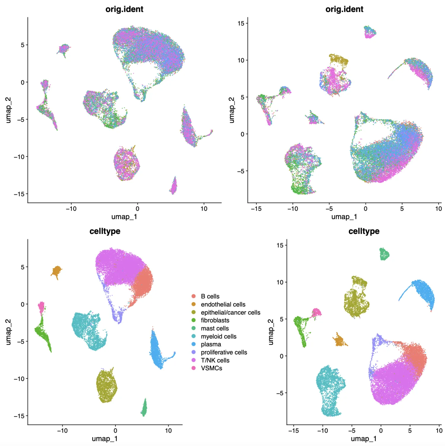
(p1+p2)/(p3+p4)
ggsave('harmony-or-not.pdf',width = 12,height = 12)
下图左边部分是harmony之后的结果,右边部分是pca的结果。我们可以发现相比于右边的结果,左边结果中细胞之间会融合更好。
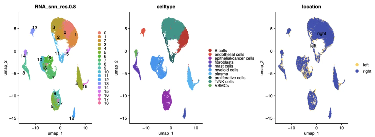
plot1 <- DimPlot(sce, reduction = "umap", group.by = "RNA_snn_res.0.8",label = T,repel = T)+
  theme(legend.key.size = unit(0.02, 'cm')) + theme(plot.title = element_text(size=12),
                                                    axis.title = element_text(size=10),
                                                    axis.text = element_text(size=10),
                                                    legend.text = element_text(size=10))
plot2 <- DimPlot(sce, reduction = "umap", group.by = "celltype",label = F,cols = color,repel = T) +
  theme(legend.key.size = unit(0.02, 'cm')) + theme(plot.title = element_text(size=12),
                                                    axis.title = element_text(size=10),
                                                    axis.text = element_text(size=10),
                                                    legend.text = element_text(size=10))
plot3 <- DimPlot(sce, reduction = "umap", group.by = "location",label = T,cols = sample(color,6),repel = T) +
  theme(plot.title = element_text(size=12),
        axis.title = element_text(size=10),
        axis.text = element_text(size=10),
        legend.text = element_text(size=10))

fig1 <- plot1|plot2|plot3
fig1
ggsave(fig1,filename = "fig1.pdf",units = "cm",width = 32,height = 1
# 排序为后续做图做准备
ord = c( "T/NK cells","plasma","myeloid cells","B cells",
"epithelial/cancer cells", "mast cells" ,"proliferative cells",
"endothelial cells","VSMCs","fibroblasts" )
ord = unique(sce.all$celltype)
all(ord %in% unique(sce.all$celltype) )
sce.all$celltype = factor(sce.all$celltype ,levels = ord)
table(sce.all$celltype)
DimPlot(sce.all)
table(Idents(sce))
table(Idents(sce.all))
if(T){
sce= sce.all
pro = 'cosg_celltype_'
library(COSG)
marker_cosg <- cosg(
sce,
groups='all',
assay='RNA',
slot='data',
mu=1,
n_genes_user=100)
save(marker_cosg,file = paste0(pro,'_marker_cosg.Rdata'))
## Top10 genes
library(dplyr)
top_10 <- unique(as.character(apply(marker_cosg$names,2,head,10)))
# width <-0.006*dim(sce)[2];width
# height <- 0.25*length(top_10)+4.5;height
width <- 15+0.5*length(unique(Idents(sce)));width
height <- 8+0.1*length(top_10);height
# levels( Idents(sce) ) = 0:length(levels( Idents(sce) ))
DoHeatmap( subset(sce,downsample=100), top_10 ,
size=3)
ggsave(filename=paste0(pro,'DoHeatmap_check_top10_markers_by_clusters.pdf') ,
# limitsize = FALSE,
units = "cm",width=width,height=height)
width <- 8+0.6*length(unique(Idents(sce)));width
height <- 8+0.2*length(top_10);height
DotPlot(sce, features = top_10 ,
assay='RNA' ) + coord_flip() +FontSize(y.text = 4)
ggsave(paste0(pro,'DotPlot_check_top10_markers_by_clusters.pdf'),
units = "cm",width=width,height=height)
## Top3 genes
top_3 <- unique(as.character(apply(marker_cosg$names,2,head,3)))
width <- 15+0.2*length(unique(Idents(sce)));width
height <- 8+0.1*length(top_3);height
DoHeatmap( subset(sce,downsample=100), top_3 ,
size=3)
ggsave(filename=paste0(pro,'DoHeatmap_check_top3_markers_by_clusters.pdf') ,
units = "cm",width=width,height=height)
width <- 8+0.2*length(unique(Idents(sce)));width
height <- 8+0.1*length(top_3);height
DotPlot(sce, features = top_3 ,
assay='RNA' ) + coord_flip()
ggsave(paste0(pro,'DotPlot_check_top3_markers_by_clusters.pdf'),width=width,height=height)
}
getwd()
pro = 'cosg_celltype_'
load(file = paste0(pro,'_marker_cosg.Rdata'))
top_10 <- unique(as.character(apply(marker_cosg$names,2,head,10)))
sce.Scale <- ScaleData(subset(sce.all,downsample=100),features = top_10 )
table(sce.Scale$celltype)
library(paletteer)
color <- c(paletteer_d("awtools::bpalette"),
paletteer_d("awtools::a_palette"),
paletteer_d("awtools::mpalette"),
paletteer_d("awtools::spalette"))
table(Idents(sce.Scale))
ll = as.list(as.data.frame(apply(marker_cosg$names,2,head,10)))
ll = ll[ord]
rmg=names(table(unlist(ll))[table(unlist(ll))>1])
ll = lapply(ll, function(x) x[!x %in% rmg])
ll
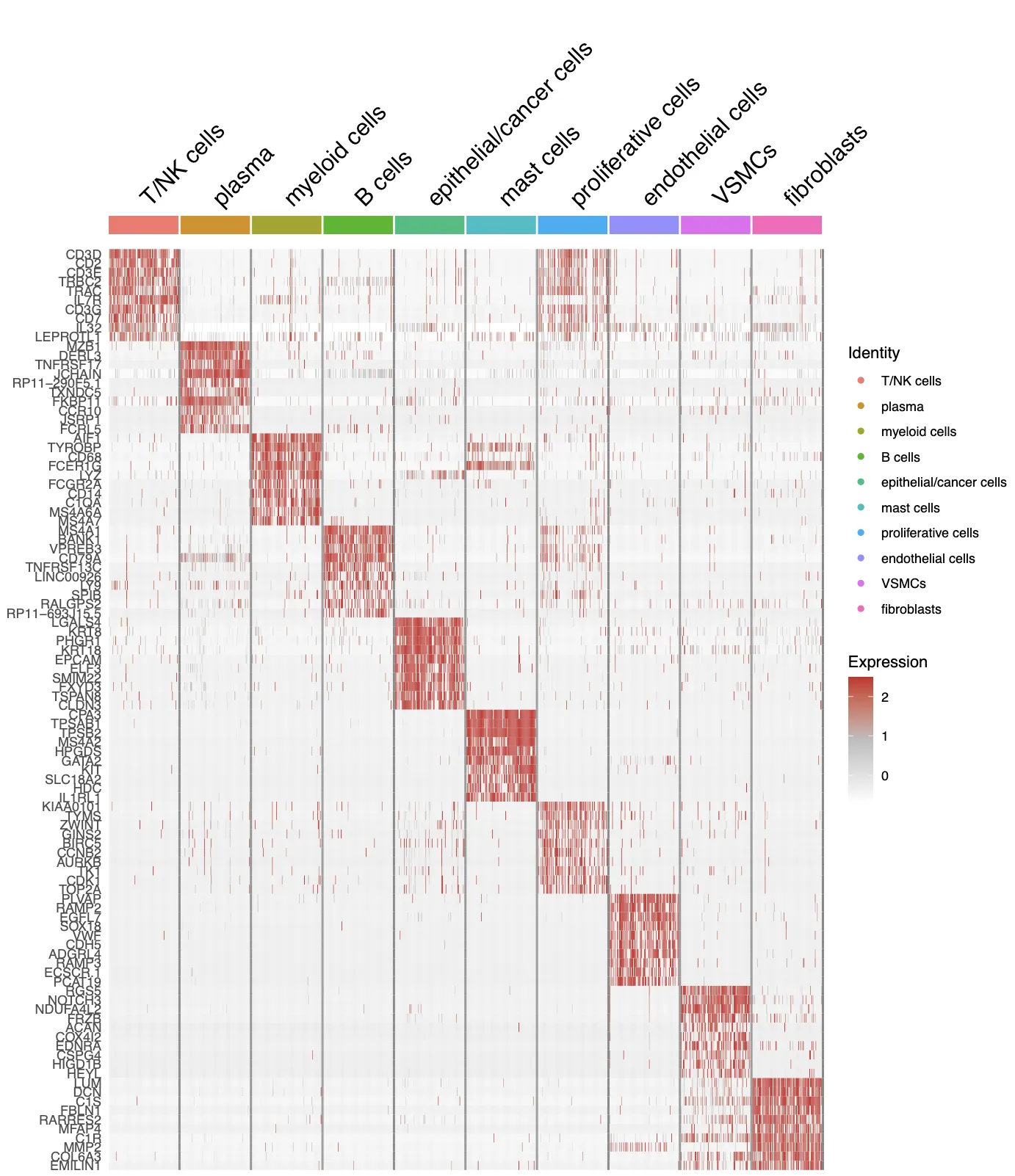
DoHeatmap(sce.Scale,
features = unlist(ll),
group.by = "celltype",
raster = F,
assay = 'RNA', label = T)+
scale_fill_gradientn(colors = c("white","grey","firebrick3"))
ggsave(filename = "fig4-top10-marker_pheatmap.pdf",units = "cm",
width = 25,height = 30)
load('../phe.Rdata')
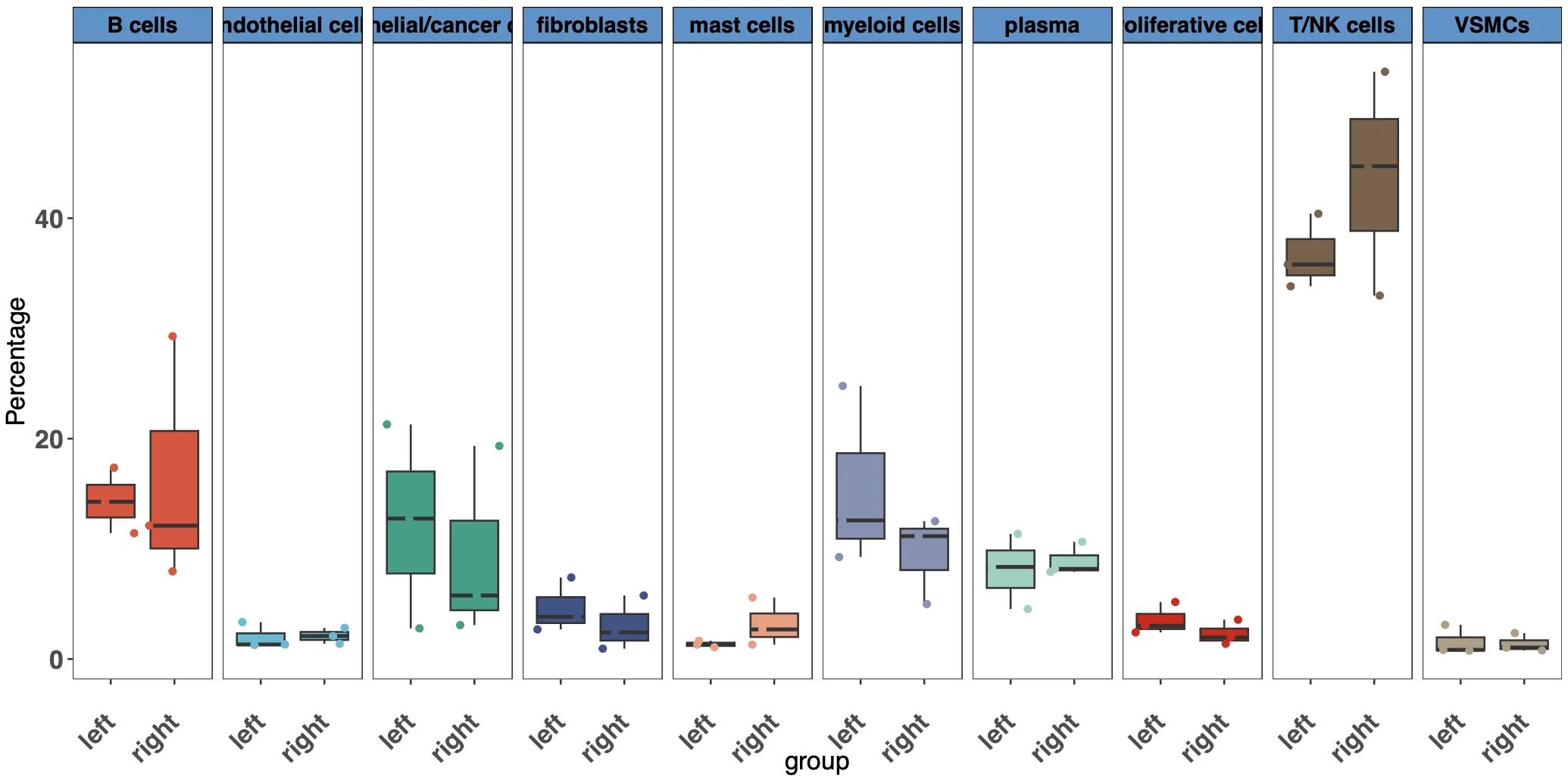
phe$group = sce$group = ifelse(sce$orig.ident %in% c("GSM5688706_WGC","GSM5688707_JCA","GSM5688708_LS-CRC3"),"left","right")
head(phe)
gplots::balloonplot(
table(phe$celltype,phe$orig.ident)
)
x = phe$orig.ident
y = phe$celltype
tbl = table(x,y)
df = dcast(as.data.frame(tbl),x~y)
ptb = round(100*tbl/rowSums(df[,-1]),2)
df = as.data.frame(ptb)
colnames(df)=c('orig.ident','celltype','Percentage')
head(df)
gpinfo=unique(phe[,c('orig.ident','group')]);gpinfo
df=merge(df,gpinfo,by='orig.ident')
head(df)
参考资料:
-
Resolving the difference between left-sided and right-sided colorectal cancer by single-cell sequencing.JCI Insight. 2022 Jan 11;7(1):e152616.
致谢:感谢曾老师以及生信技能树团队全体成员。更多精彩内容可关注公众号:生信技能树,单细胞天地,生信菜鸟团等公众号。
注:若对内容有疑惑或者有发现明确错误的朋友,请联系后台(欢迎交流)。更多相关内容可关注公众号:生信方舟
- END -


 816
816

 被折叠的 条评论
为什么被折叠?
被折叠的 条评论
为什么被折叠?
 到【灌水乐园】发言


