MCMC: Metropolis-Hastings, Gibbs and slice sampling

从标题中即已看出，Metropolis-Hastings、Gibbs and slice sampling是MCMC（基于马尔科夫链的蒙特卡洛采样算法）的变体及改进算法。

With MCMC, we draw samples from a (simple) proposal distribution so that each draw depends only on the state of the previous draw (i.e. the samples form a Markov chain).

The nice thing is that this target distribution only needs to be proportional to the posterior distribution, which means we don’t need to evaluate the potentially intractable marginal likelihood, which is just a normalizing constant. We can find such a target distribution easily, since posterior $\propto$ likelihood $\times$ prior.

Metropolis-Hastings

To carry out the Metropolis-Hastings algorithm, we need to draw random samples from the folllowing distributions：

• 标准均匀分布$\sim U(0, 1)$

• a proposal distriution $p(x)$ that we choose to be $\mathcal{N}(0,\sigma)$

• the target distribution $g(x)$ which is proportional to the posterior probability

Given an initial guess for $\theta$ with positive probability of being drawn, the Metropolis-Hastings algorithm proceeds as follows

• step 1：Choose a new proposed value ($\theta_p$) such that $\theta_p=\theta+\Delta\theta$ where $\Delta\theta\sim \mathcal{N}(0,\sigma)$

• step 2: Caluculate the ratio
  

  $$\rho=\frac{g(\theta_p|X)}{g(\theta|X)}$$
  where $g$ is the posterior probability.

If the proposal distribution $p(\cdot)$ is not symmetrical（$p(\theta_p|\theta)\neq p(\theta|\theta_p)$）, we need to weight the accceptanc probablity to maintain detailed balance (reversibilty) of the stationary distribution, and instead calculate:

$$\rho = \frac{g(\theta_p|X)p(\theta|\theta_p)}{g(\theta|X)p(\theta_p|\theta)}$$

Since we are taking ratios, the denominator cancels any distribution proporational to $g$ will also work - so we can use

$$\rho = \frac{p(X|\theta_p)p(\theta_p)}{p(X|\theta)p(\theta)}$$

If $\rho≥1$, then set $\theta=\theta_p$

If $\rho<1$, then set$\theta=\theta_p$ with probability $\rho$, otherwise set $\theta=\theta$ (this is where we use the standard uniform distribution$\sim U(0, 1)$)

• step3：也即，$\rho=\min\{\frac{p(X|\theta_p)p(\theta_p)}{p(X|\theta)p(\theta)}, 1\}$，if $u\sim U(0, 1)<\rho$, $\theta=\theta_p$（进行跳转），else $\theta=\theta$.

• step 4：repeat the earlier steps

import numpy as np
import scipy.stats as st
import matplotlib.pyplot as plt

n, k = 100, 61
a, b = 10, 10 
like = st.binom
prior = st.beta(a, b)
                # poster = st.beta(a+k, b+n-k)
def target(prior, like, n, k, theta):
    return 0 if theta < 0 or theta > 1 else prior.pdf(theta)*like(n, theta).pmf(k)

naccept = 0
niters = 10**4
theta = 0.001
samples = np.zeros(niters+1)
samples[0] = theta
sigma = .3
for i in range(niters):
    theta_p = theta + st.norm(0, sigma).rvs()
    rho = min(target(prior, like, n, k, theta_p)/target(prior, like, n, k, theta), 1)
    u = st.uniform(0, 1).rvs()
    if u < rho:
        naccept += 1
        theta = theta_p
    samples[i+1] = theta
nmcmc = len(samples)//2
print('efficiency', naccept/niters)
                # 0.1833
poster = st.beta(a+k, b+n-k)

thetas = np.arange(0, 1, .001)

plt.hist(prior.rvs(nmcmc), 40, histtype='step', c='b', label='distribution of prior samples')
plt.hist(samples[nmcmc:], 40, histtype='step', c='r', label='distribution of posterior samples')
plt.plot(thetas, poster.pdf(thetas), ls='--', c='r', label='True posterior')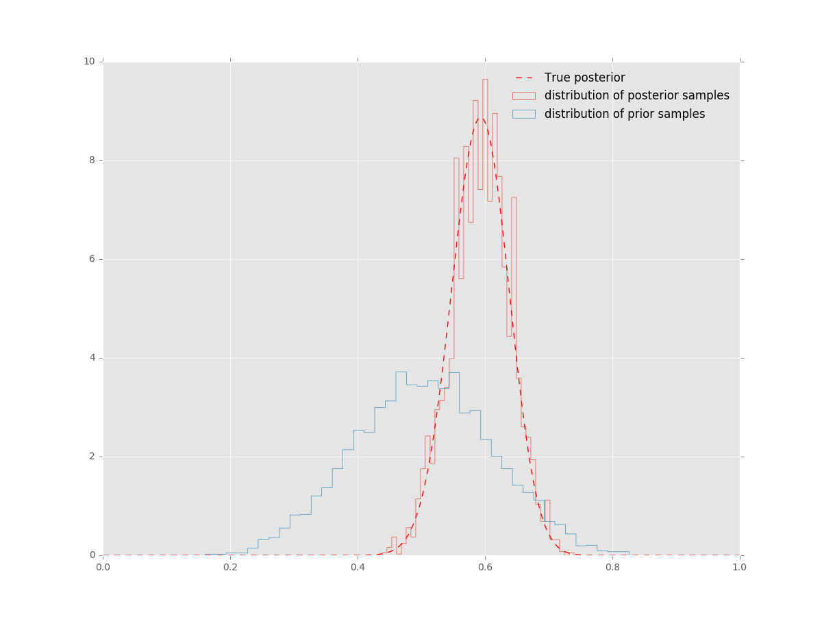

Gibbs sampler

Suppose we have a vector of parameters $θ=(θ_1,θ_2,…,θ_k)$, and we want to estimate the joint posterior distribution $p(θ|X)$. Suppose we can find and draw random samples from all the conditional distributions.

$$\begin{split} \begin{array}{c} p(\theta_1|\theta_2,\dots,\theta_k,X)\\ p(\theta_2|\theta_1,\dots,\theta_k,X)\\ \ldots\\ p(\theta_k|\theta_1,\theta_2,\dots,X)\\ \end{array} \end{split}$$
With Gibbs sampling, the Markov chain is constructed by sampling from the conditional distribution for each parameter $θ_i$ in turn, treating all other parameters as observed. When we have finished iterating over all parameters, we are said to have completed one cycle of the Gibbs sampler. Where it is difficult to sample from a conditional distribution, we can sample using a Metropolis-Hastings algorithm instead - this is known as Metropolis wihtin Gibbs.

Gibbs sampling is a type of random walk through parameter space, and hence can be thought of as a Metroplish-Hastings algorithm with a special proposal distribution（被认为是一种具有特定proposal distribution的M-H算法）. At each iteration in the cycle, we are drawing a proposal for a new value of a particular parameter, where the propsal distribution is the conditional posterior probability of that parameter. This means that the proposal move is always accepted. Hence, if we can draw samples from the conditional distributions, Gibbs sampling can be much more efficient than regular Metropolis-Hastings.

使用解析解，如果存在的话

from functools import reduce
from operator import mul
import numpy as np
import matplotlib.pyplot as plt
import scipy.stats as st

def comb(N, k):
    return reduce(mul, range(N-k+1, N+1))//reduce(mul, range(1, k+1))
                        # 组合数C_N^k的计算
def bern(theta, N, k):
    return comb(N, k)*theta**k*(1-theta)**(N-k)
                        # 二项分布，或者叫n重伯努利试验
def bern2(theta1, theta2, N1, N2, k1, k2):
    return bern(theta1, N1, k1)*bern(theta2, N2, k2)
                        # '二维'伯努利分布

def make_thetas(xmin, xmax, n):
    xs = np.linspace(xmin, xmax, n)
    widths = (xs[1:]-xs[:-1])/2
    thetas = xs[:-1]+widths
    return thetas

def make_plots(X, Y, prior, lik, poster, projection=None):
    fig, ax = plt.subplots(1, 3, subplot_kw=dict(projection=projection, aspect='equal'), figsize=(12, 9))
    if projection=='3d':
            # 需要引入
            # from mpl_toolkits.mplot3d import Axes3D
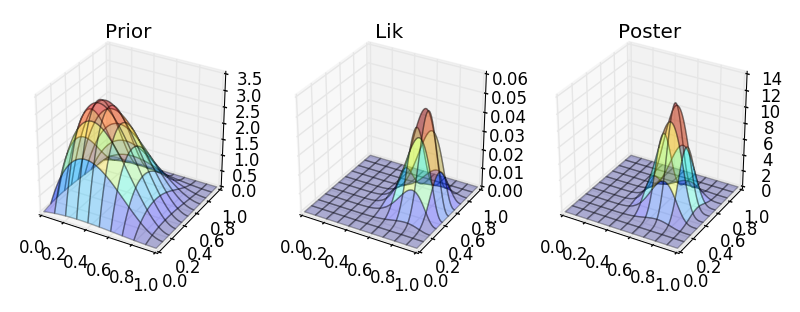
        ax[0].plot_surface(X, Y, prior, alpha=.3, cmap=plt.cm.jet)
        ax[1].plot_surface(X, Y, lik, alpha=.3, cmap=plt.cm.jet)
        ax[2].plot_surface(X, Y, poster, alpha=.3, cmap=plt.cm.jet)
    else:
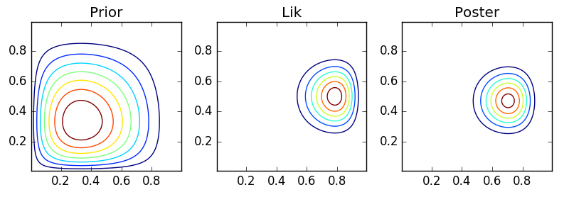
        ax[0].contour(X, Y, prior)
        ax[1].contour(X, Y, lik)
        ax[2].contour(X, Y, poster)
    ax[0].set_title('Prior')
    ax[1].set_title('Lik')
    ax[2].set_title('Poster')
    plt.tight_layout()
    plt.show()

thetas1 = make_thetas(0, 1, 101)
thetas2 = make_thetas(0, 1, 101)
X, Y = np.meshgrid(thetas1, thetas2)

a, b = 2, 3
N1, k1 = 14, 11
N2, k2 = 14, 7

prior = st.beta(a, b).pdf(X)*st.beta(a, b).pdf(Y)
lik = bern2(X, Y, N1, N2, k1, k2)
poster = st.beta(a+k1, b+N1-k1).pdf(X)*st.beta(a+k2, b+N2-k2).pdf(Y)
make_plots(X, Y, prior, lik, poster)
make_plots(X, Y, prior, lik, poster, '3d')