


问题
考虑如下的数据集:
x,y
是观测到的变量(observed variables),
y
的误差存放在数组
x = np.array([ 0,  3,  9, 14, 15, 19, 20, 21, 30, 35,
              40, 41, 42, 43, 54, 56, 67, 69, 72, 88])
y = np.array([33, 68, 34, 34, 37, 71, 37, 44, 48, 49,
              53, 49, 50, 48, 56, 60, 61, 63, 44, 71])
e = np.array([ 3.6, 3.9, 2.6, 3.4, 3.8, 3.8, 2.2, 2.1, 2.3, 3.8,
               2.2, 2.8, 3.9, 3.1, 3.4, 2.6, 3.4, 3.7, 2.0, 3.5])
对数据集作如下的可视化工作:
import matplotlib.pyplot as plt
plt.errorbar(x, y, e, fmt='ok', ecolor='gray')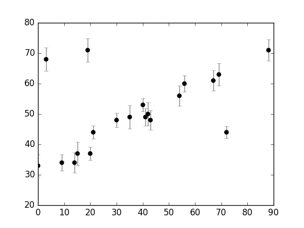
我们的工作即是找到能够拟合这些点的一条直线。视觉上很容易看出这些点中存在离群点(outliers)。
矩阵以及最小平方误差的形式
我们可使用最大似然估计(Maximum Likelihood Estimation)的策略寻找这样的点:
我们首先定义一个简单的线性模型(Linear Model),
y^(xi|θ)=θ0+θ1x
在这一模型之下,我们可计算每一点所对应的高斯似然:
p(xi,yi,ei|θ)∝exp[−(yi−y^(xi|θ))22e2i]
全体样本的对数似然为:
logL(D|θ)=const−∑i=1n(yi−y^(xi|θ))22e2i
通常的最优化函数一般是最小化某一损失函数(Loss Function)(比如,scipy库下的optimize.fmin()),我们将最大化该数据集的高斯似然转换为最小化如下的损失函数:
loss=∑i=1n(yi−y^(xi|θ))22e2i
这一损失函数的形式即是著名的 Squared Loss (平方误差),也即我们可从高斯似然中推导出平方误差的形式。
我们可通过两种方法进行最优化损失函数的求解,:
- 使用公式:
θ=(XTX)−1XTy
其中 X 是样本矩阵增广的形式,也即第一列为全1.
x_aug = np.hstack((np.ones((len(x), 1)), x.reshape((-1, 1))))/np.dot(e.reshape((-1, 1)), np.ones((1, 2)))
p_inv = np.dot(np.linalg.inv(np.dot(x_aug.T, x_aug)), x_aug.T)
theta0 = np.dot(p_inv, y/e)- 调用最优化工具箱函数
def squared_loss(theta, x, y, e):
    return ((y-(theta[0]+theta[1]*x))/e)**2/2.sum()
import scipy
theta1 = optimize.fmin(theta, x0=(0, 0), args=(x, y, z), disp=False)
平方误差函数的形式(以及实践)均说明这种线性拟合的方法,对离群点较为敏感。
下面给出两种解决方案,分别是频率主义学派的Huber Loss(对噪声敏感的根源在于平方误差损失函数,改变损失函数的形式自然是一种可以想见的解决方案),以及是贝叶斯主义学派的Nuisance Parameters。
Huber Loss
def huber_loss(theta, x, y, e, delta=3):
    diff = abs(y-(theta[0]+theta[1]*x))
    return ((diff < delta)*diff**2/2+(diff >= delta)*delta*(diff-delta/2)).sum()
theta[2] = optimize.fmin(huber_loss, x0=(0, 0), args=(x, y, e), disp=False)
Bayesian的方式:Nuisance Parameters
P({xi},{yi},{ei}|θ,{gi},σB)=gi2πe2i−−−−√exp[−(y^(xi|θ)−yi)22e2i]+1−gi2πσ2B−−−−−√exp(−(y^(xi|θ)−yi)22σ2B)
def log_prior(theta):
    if all(theta[2:] > 0) and all(theta[2:]<1):
        return 0
    else:
        return -np.inf

def log_likelihood(theta, x, y, e, sigma_B):
    g = np.clip(theta[2:], 0, 1)
    diff = y-(theta[0]+theta[1]*x)
    logl1 = np.log(g)-np.log(2*np.pi*e**2)/2-(diff/e)**2/2
    logl2 = np.log(1-g)-np.log(2*np.pi*sigma_B**2)/2-(diff/e)**2/2
    return np.logaddexp(logl1, logl2)

def log_posterior(theta, x, y, e, sigma_B):
    return log_prior(theta)+log_likelihood(x, y, e, sigma_B)
import emcee
ndim = 2+len(x)
nwalkers = 50
nburn = 10000
nsteps = nburn + nburn/2
p0 = np.zeros(nwalkers*ndim).reshape((nwalkers, ndim))
p0[:, :2] = np.random.normal(theta[1], 1, (nwalkers, 2))
p0[:, 2:] = np.random.uniform(0, 1, (nwalkers, ndim-2))
sampler = emcee.EnsembleSampler(nwalkers, ndim, log_posterior, args=(x, y, e, 50))
sampler.run_mcmc(p0, nsteps)
samples = sampler.chain[:, nburn:, :].reshape((-1, ndim))
thetas = np.mean(samples, 0)
theta[3] = thetas[:2]
outliers = (thetas[2:] < .5)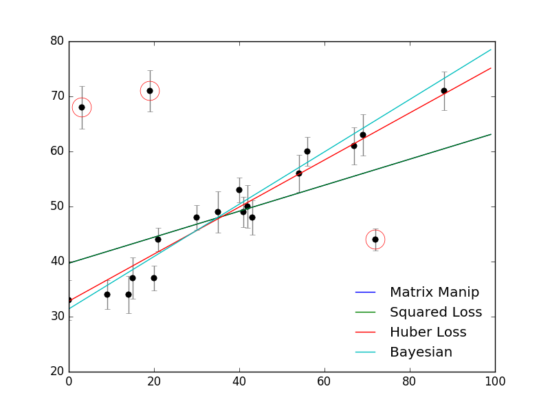


 919
919

 被折叠的 条评论
为什么被折叠?
被折叠的 条评论
为什么被折叠?
 到【灌水乐园】发言


