贝叶斯分析——从数值积分到MCMC

Analytical solution

Numerical integration

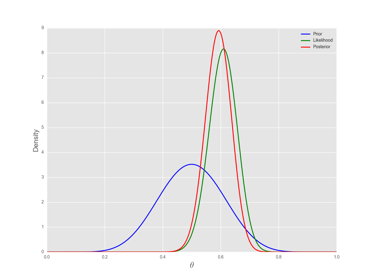
One simple way of numerical integration is to estimate the values on a grid of values for $\theta$. To calculate the posterior, we find the prior and the likelhood for each value of $\theta$, and for the marginal likelhood, we replace the integral with the equivalent sum

$$p(X)=\sum_{\theta^*} P(\theta^*)P(X|\theta^*)$$

One advantage of this is that the prior does not have to be conjugate (although the example below uses the same beta prior for ease of comaprsion), and so we are not restricted in our choice of an approproirate prior distribution. For example, the prior can be a mixture distribution or estimated empirically from data. For example, the prior can be a mixture distribution or estimated empirically from data. The disadvantage, of course, is that this is computationally very expenisve when we need to esitmate multiple parameters, since the number of grid points grows as $O(n^d)$, wher $n$ defines the grid resolution（thetas=np.arange(0, 1, .001)） and $d$ is the size of $\theta=[\theta[0], \theta[1], g_i]$.

import numpy as np
import scipy.stats as st
import matplotlib.pyplot as plt

a, b = 10, 10
n, k = 100, 61

thetas = np.arange(0, 1, .001)
prior = st.beta(a, b)
poster = prior.pdf(thetas) * st.binom(n, thetas).pmf(k)
                    # 
poster /= (poser.sum()/len(thetas))
                    # ∑p(θ)p(x|θ)
plt.plot(thetas, prior.pdf(thetas), 'b', lw=2, label='Prior')
plt.plot(thetas, n*st.binom(n, thetas).pmf(k), 'g', lw=2, label='Likelihood')
plt.plot(thetas, poster, 'r', lw=2, label='Posterior')