


延续上一篇推文:转录组8种免疫浸润分析方法整理(https://mp.weixin.qq.com/s/sy-HT1znQYTcktN3ef-djw)
这次来整理和学习一下IOBR这个功能强大的R包
IOBR(Immuno-Oncology Biological Research,免疫肿瘤学生物研究)这个R包整合了8种已发表的方法(CIBERSORT、TIMER、xCell、MCPcounter、ESTIMATE、EPIC、IPS和quanTIseq),用于解析肿瘤微环境的背景信息。
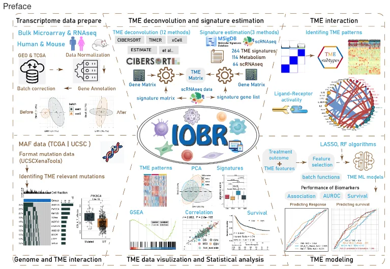
此外,开发者还收集了264个已发表的基因集签名,涵盖了肿瘤微环境、肿瘤代谢、m6A、外泌体、微卫星不稳定性和三级淋巴结构。通过运行signature_collection_citation函数,可以获取这些基因集签名的来源文献,而signature_collection函数则返回所有给定签名的详细基因。IOBR使用了三种计算方法来计算签名得分,包括PCA、z-score和ssGSEA。值得注意的是,IOBR还收集并使用了多种方法进行变量转换、可视化、批量生存分析、特征选择和统计分析。该包支持批量分析和结果可视化。
综合来看,IOBR是一个重点解析肿瘤微环境且不仅限于此的强大的工具R包。
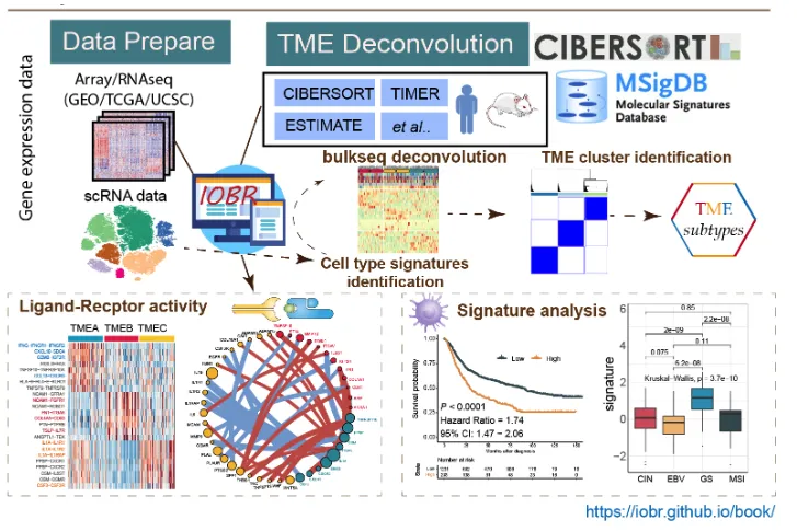
这个是目前IOBR更新之后的内容,从图片中就可以看出IOBR增加了更多有趣的东西。首先是可输入的数据也从单纯普通的RNA数据进入了单细胞时代。此外增加了多种新的分析内容,包括了单细胞数据的配体和受体活性网络分析,去卷积之后的肿瘤微环境聚类分群,还有sigature分析等。
本次重点探索一下多种转录组免疫浸润分析。
分析流程
1、加载数据
rm(list = ls())
load("~/Desktop/data/combat.Rdata")
head(exp)[1:4,1:4]
#           GSM3106326 GSM3106327 GSM3106328 GSM3106329
# LINC01128   8.000049   8.044479   7.311868   7.610713
# SAMD11      7.499611   7.562370   7.412649   7.239141
# KLHL17      7.662076   7.672331   7.627330   7.564212
# PLEKHN1     7.666884   7.889537   7.640606   7.746440
head(pd)
#                                                title                  samples   GSE_num group
# GSM3106326 Pulmonary arterial hypertension patient 1   idiopathic PAH patient GSE113439   PAH
# GSM3106327 Pulmonary arterial hypertension patient 2 patient with PAH and CHD GSE113439   PAH
# GSM3106328 Pulmonary arterial hypertension patient 3 patient with PAH and CTD GSE113439   PAH
# GSM3106329 Pulmonary arterial hypertension patient 4 patient with PAH and CHD GSE113439   PAH
# GSM3106330 Pulmonary arterial hypertension patient 5   idiopathic PAH patient GSE113439   PAH
# GSM3106331 Pulmonary arterial hypertension patient 6   idiopathic PAH patient GSE113439   PAH

identical(rownames(pd),colnames(exp))
# [1] TRUE

library(IOBR)
tme_deconvolution_methods
      #  MCPcounter               EPIC              xCell          CIBERSORT CIBERSORT Absolute
      # "mcpcounter"             "epic"            "xcell"        "cibersort"    "cibersort_abs"
      #          IPS           ESTIMATE                SVR               lsei              TIMER
      #        "ips"         "estimate"              "svr"             "lsei"            "timer"
      #    quanTIseq
      #  "quantiseq"
内置了多种免疫分析方法:mcpcounter,epic,xcell,cibersort,cibersort_abs,ips,ESTIMATE,SVR,lsei,TIMER,quanTIseq
2、cibersort
ciber_res<-deconvo_tme(eset = exp, method = "cibersort",
arrays = TRUE, perm = 100 )
ciber_res
# # A tibble: 132 × 26
# ID B_cells_naive_CIBERSORT B_cells_memory_CIBERSORT Plasma_cells_CIBERSORT T_cells_CD8_CIBERSORT
# <chr> <dbl> <dbl> <dbl> <dbl>
# 1 GSM3106326 0.0142 0 0.0698 0.0456
# 2 GSM3106327 0.0281 0 0.00704 0.0218
# 3 GSM3106328 0.0309 0 0.0257 0.0224
# 4 GSM3106329 0.0335 0 0.0355 0.0386
# 5 GSM3106330 0.0471 0 0.0263 0.0666
# 6 GSM3106331 0.0441 0 0.0220 0
# 7 GSM3106332 0.0205 0 0.118 0.133
# 8 GSM3106333 0.0370 0 0.0307 0.0805
# 9 GSM3106334 0.0537 0 0.0501 0.0218
# 10 GSM3106335 0 0 0.0210 0.0196
# # ℹ 122 more rows
# # ℹ 21 more variables: T_cells_CD4_naive_CIBERSORT <dbl>, T_cells_CD4_memory_resting_CIBERSORT <dbl>,
# # T_cells_CD4_memory_activated_CIBERSORT <dbl>, T_cells_follicular_helper_CIBERSORT <dbl>,
# # `T_cells_regulatory_(Tregs)_CIBERSORT` <dbl>, T_cells_gamma_delta_CIBERSORT <dbl>,
# # NK_cells_resting_CIBERSORT <dbl>, NK_cells_activated_CIBERSORT <dbl>, Monocytes_CIBERSORT <dbl>,
# # Macrophages_M0_CIBERSORT <dbl>, Macrophages_M1_CIBERSORT <dbl>, Macrophages_M2_CIBERSORT <dbl>,
# # Dendritic_cells_resting_CIBERSORT <dbl>, Dendritic_cells_activated_CIBERSORT <dbl>, …
# # ℹ Use `print(n = ...)` to see more rows
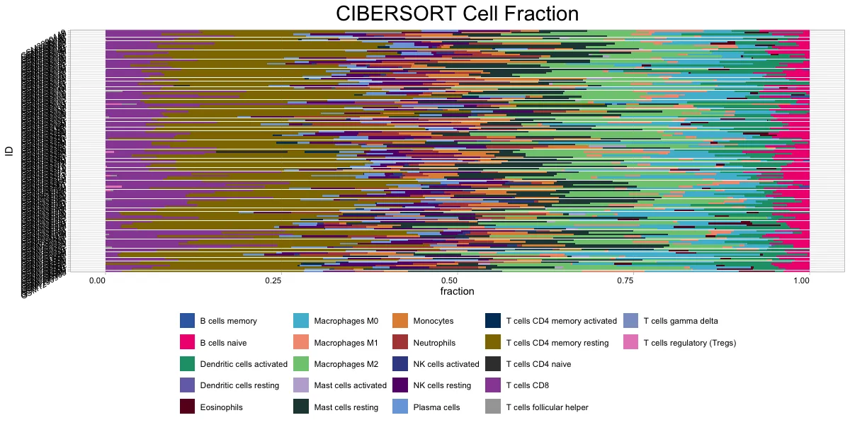
ciber_plot <- cell_bar_plot(input = ciber_res, features = colnames(ciber_res)[2:23],
title = "CIBERSORT Cell Fraction")
里面内置了cell_bar_plot函数进行快速绘图
3.epic
epic_res <- deconvo_tme(eset = exp, method = "epic", arrays = TRUE)
epic_res
# # A tibble: 132 × 9
#    ID       Bcells_EPIC CAFs_EPIC CD4_Tcells_EPIC CD8_Tcells_EPIC Endothelial_EPIC Macrophages_EPIC NKcells_EPIC
#    <chr>          <dbl>     <dbl>           <dbl>           <dbl>            <dbl>            <dbl>        <dbl>
#  1 GSM3106…      0.0266   0.00939           0.145          0.0877            0.111          0.00673     2.14e-10
#  2 GSM3106…      0.0258   0.00795           0.145          0.0867            0.109          0.00684     2.01e-10
#  3 GSM3106…      0.0281   0.00793           0.145          0.0889            0.109          0.00672     1.71e-10
#  4 GSM3106…      0.0284   0.00909           0.143          0.0867            0.109          0.00664     1.63e-10
#  5 GSM3106…      0.0264   0.00799           0.144          0.0867            0.115          0.00638     1.53e- 9
#  6 GSM3106…      0.0292   0.00783           0.148          0.0855            0.108          0.00668     1.22e-10
#  7 GSM3106…      0.0261   0.00928           0.139          0.0899            0.115          0.00646     7.15e-10
#  8 GSM3106…      0.0253   0.00854           0.139          0.0894            0.106          0.00674     8.18e-10
#  9 GSM3106…      0.0325   0.00857           0.151          0.0893            0.106          0.00676     1.27e-10
# 10 GSM3106…      0.0263   0.00809           0.132          0.0841            0.106          0.00640     1.01e- 9
# # ℹ 122 more rows
# # ℹ 1 more variable: otherCells_EPIC <dbl>
# # ℹ Use `print(n = ...)` to see more rows
epic_plot <- cell_bar_plot(input = epic_res, features = colnames(epic_res)[2:9],
                            title = "EPIC Cell Fraction")
4.quantiseq
quantiseq_res <- deconvo_tme(eset = exp, tumor = F,
                             arrays = TRUE, scale_mrna = TRUE, method = "quantiseq")
quantiseq_res
# # A tibble: 132 × 12
#    ID         B_cells_quantiseq Macrophages_M1_quantiseq Macrophages_M2_quantiseq Monocytes_quantiseq
#    <chr>                  <dbl>                    <dbl>                    <dbl>               <dbl>
#  1 GSM3106326            0.0561                    0.195                   0.0910             0.00835
#  2 GSM3106327            0.0462                    0.417                   0.0557             0
#  3 GSM3106328            0.0640                    0.194                   0.0830             0.0118
#  4 GSM3106329            0.0707                    0.182                   0.142              0.0433
#  5 GSM3106330            0.0501                    0.257                   0.0887             0
#  6 GSM3106331            0.0480                    0.424                   0.0940             0
#  7 GSM3106332            0.0638                    0.183                   0.0849             0.122
#  8 GSM3106333            0.0564                    0.277                   0.0878             0
#  9 GSM3106334            0.0713                    0.272                   0.106              0
# 10 GSM3106335            0.0532                    0.203                   0.111              0.0201
# # ℹ 122 more rows
# # ℹ 7 more variables: Neutrophils_quantiseq <dbl>, NK_cells_quantiseq <dbl>, T_cells_CD4_quantiseq <dbl>,
# #   T_cells_CD8_quantiseq <dbl>, Tregs_quantiseq <dbl>, Dendritic_cells_quantiseq <dbl>,
# #   Other_quantiseq <dbl>
# # ℹ Use `print(n = ...)` to see more rows
quantiseq_plot <- cell_bar_plot(input = quantiseq_res, features = colnames(quantiseq_res)[2:12],
                            title = "Quantiseq Cell Fraction")
5. MCPcounter
mcpcounter_res <- deconvo_tme(eset = exp, method = "mcpcounter")
mcpcounter_res
# # A tibble: 132 × 11
# ID T_cells_MCPcounter CD8_T_cells_MCPcounter Cytotoxic_lymphocytes_MCPcoun…¹ B_lineage_MCPcounter
# <chr> <dbl> <dbl> <dbl> <dbl>
# 1 GSM3106326 7.41 7.03 6.92 6.88
# 2 GSM3106327 7.65 7.02 7.51 6.75
# 3 GSM3106328 8.02 6.92 6.55 7.04
# 4 GSM3106329 7.55 6.72 6.68 7.00
# 5 GSM3106330 7.61 7.00 6.56 6.71
# 6 GSM3106331 7.92 6.89 6.53 7.17
# 7 GSM3106332 7.30 7.04 6.75 6.54
# 8 GSM3106333 7.50 7.14 6.90 6.61
# 9 GSM3106334 8.11 7.26 7.05 8.03
# 10 GSM3106335 6.88 6.94 6.77 6.71
# # ℹ 122 more rows
# # ℹ abbreviated name: ¹Cytotoxic_lymphocytes_MCPcounter
# # ℹ 6 more variables: NK_cells_MCPcounter <dbl>, Monocytic_lineage_MCPcounter <dbl>,
# # Myeloid_dendritic_cells_MCPcounter <dbl>, Neutrophils_MCPcounter <dbl>,
# # Endothelial_cells_MCPcounter <dbl>, Fibroblasts_MCPcounter <dbl>
# # ℹ Use `print(n = ...)` to see more rows
6. xCELL
xCELL_res <- deconvo_tme(eset = exp, method = "xcell",arrays = TRUE)
# >>> Running xCell
# [1] "Num. of genes: 10365"
# Error in GSVA::gsva(expr, signatures, method = "ssgsea", ssgsea.norm = FALSE) :
#   Calling gsva(expr=., gset.idx.list=., method=., ...) is defunct; use a method-specific parameter object (see '?gsva').
这里的xCell用到了gsva,然后gsva这个函数进行了更新,但IOBR应该还没有更新~ 如果需要分析的话需要加载xCell的原始函数分析。
7. TIMER
#这里导入的group_list必须是TIMER能够识别的,比如TCGA中33肿瘤类型
TIMER_res <- deconvo_tme(eset = exp, method = "timer",group_list = group_list)
8. estimate
estimate_res <- deconvo_tme(eset = exp, method = "estimate")
estimate_res
# # A tibble: 132 × 5
#    ID         StromalScore_estimate ImmuneScore_estimate ESTIMATEScore_estimate TumorPurity_estimate
#    <chr>                      <dbl>                <dbl>                  <dbl>                <dbl>
#  1 GSM3106326                 1164.                1925.                  3088.                0.490
#  2 GSM3106327                 1099.                2154.                  3253.                0.469
#  3 GSM3106328                 1213.                2174.                  3387.                0.452
#  4 GSM3106329                 1430.                1805.                  3236.                0.471
#  5 GSM3106330                 1009.                1659.                  2668.                0.543
#  6 GSM3106331                  879.                1854.                  2733.                0.535
#  7 GSM3106332                 1508.                1261.                  2770.                0.531
#  8 GSM3106333                 1335.                1855.                  3189.                0.477
#  9 GSM3106334                 1483.                2314.                  3797.                0.397
# 10 GSM3106335                  562.                1615.                  2177.                0.602
# # ℹ 122 more rows
# # ℹ Use `print(n = ...)` to see more rows
9. IPS
ips_res <- deconvo_tme(eset = exprSet, method = "ips", plot= F)
head(ips_res)
# # A tibble: 6 × 7
#   ID         MHC_IPS EC_IPS SC_IPS  CP_IPS AZ_IPS IPS_IPS
#   <chr>        <dbl>  <dbl>  <dbl>   <dbl>  <dbl>   <dbl>
# 1 GSM3106326    1.11 -0.330    NaN -0.264   0.515       2
# 2 GSM3106327    1.16 -0.430    NaN -0.234   0.493       2
# 3 GSM3106328    1.19 -0.406    NaN -0.0991  0.680       2
# 4 GSM3106329    1.06 -0.374    NaN -0.0446  0.642       2
# 5 GSM3106330    1.16 -0.252    NaN -0.0968  0.808       3
# 6 GSM3106331    1.06 -0.348    NaN -0.0608  0.655       2
值得一提的是这个IPS,其是指immunophenotype (免疫表型评分)。 里面一共评估四个主要参数分别是:MHC分子(MHC molecules,MHC) ,免疫调节分子(Immunomodulators,CP) ,效应细胞(Effector cells,EC) ,抑制细胞(Suppressor cells,SC) 。使用者可以根据得到的结果联合生存数据/临床参数分析。
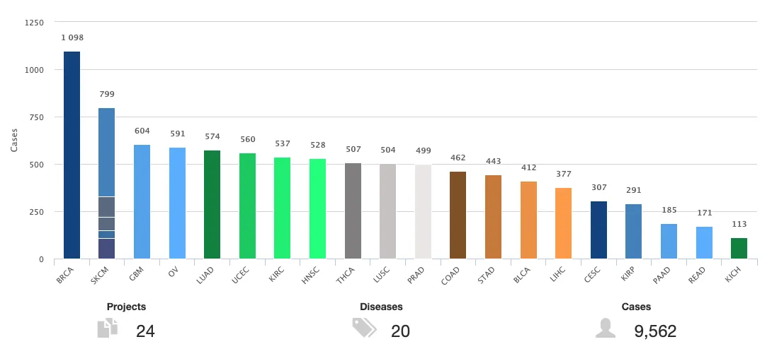
如果研究内容是如下图中的这20种实体瘤数据可以直接去TCIA官网下载(链接在参考资料)。如果是TCIA中没有的癌种,或者其他的肿瘤数据可以使用IOBR预测评分。
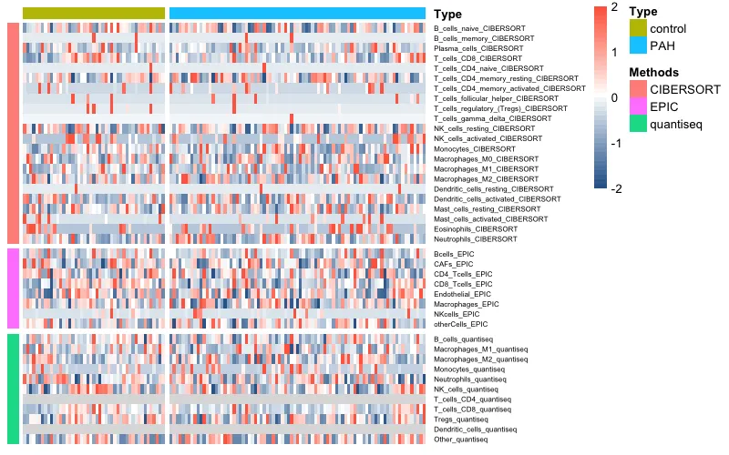
10.1、pheatmap热图
library(pheatmap)
library(RColorBrewer)
library(tidyverse)
library(gplots)
#整合数据-挑选了三个绝对丰度的结果
data_total <- cbind(ciber_res[,-c(24:26)],epic_res[,-1],quantiseq_res[,-1])
data_total <- as.data.frame(t(data_total))
colnames(data_total) <- data_total[1,]
data_total <- dplyr::slice(data_total,-1)
head(data_total)[1:5,1:5]
#                               GSM3106326   GSM3106327   GSM3106328   GSM3106329   GSM3106330
# B_cells_naive_CIBERSORT     0.0142251364 0.0281206504 0.0308628121 0.0335228312 0.0471364646
# B_cells_memory_CIBERSORT     0.000000000  0.000000000  0.000000000  0.000000000  0.000000000
# Plasma_cells_CIBERSORT       0.069795054  0.007039938  0.025673056  0.035549703  0.026348560
# T_cells_CD8_CIBERSORT        0.045625893  0.021829211  0.022410222  0.038619601  0.066552186
# T_cells_CD4_naive_CIBERSORT   0.00000000   0.00000000   0.00000000   0.00000000   0.00000000

# 检查数据类型是否正确转换为数值型
data_total <- data_total %>% mutate_all(as.numeric)

# 数据标准化-方法1
# stand_fun <- function(indata=NULL, halfwidth=NULL, centerFlag=T, scaleFlag=T) {
#                   outdata=t(scale(t(indata), center=centerFlag, scale=scaleFlag))
#                   if (!is.null(halfwidth)) {
#                      outdata[outdata > halfwidth] = halfwidth
#                      outdata[outdata < (-halfwidth)] = -halfwidth
#   }
#   return(outdata)
# }
#data_total <- stand_fun(data_total,halfwidth = 2)

# 标准化-方法2
data_total <- scale(data_total)

# 重新对列进行排序
# group_list 是一个向量,表示每个样本的类型(PAH 或 control)
sorted_index <- order(group_list, decreasing = FALSE)
# 使用排序索引对 data_total 重新排序列
data_total <- data_total[, sorted_index]
# 重新对 group_list 进行排序,以匹配列的顺序
group_list <- group_list[sorted_index]

# 创建注释
# 列注释
annCol <- data.frame(Type = group_list,
                     row.names = colnames(data_total),
                     stringsAsFactors = FALSE)
# 行注释
# 从行名中提取方法
methods <- sub('.*_', '', rownames(data_total))
# 创建行注释数据框
annRow <- data.frame(Methods = factor(methods, levels = unique(methods)),
                     row.names = rownames(data_total),
                     stringsAsFactors = FALSE)


# 调整颜色梯度
breaksList = seq(-5, 5, by = 0.1)
colors <- colorRampPalette(c("#336699", "white", "tomato"))(length(breaksList))

# 绘制热图
pheatmap(data_total,
         annotation_col = annCol,
         annotation_row = annRow,
         color = colors,
         breaks = breaksList,
         cluster_rows = FALSE,
         cluster_cols = FALSE,
         show_rownames = TRUE,
         show_colnames = FALSE,
         gaps_col = cumsum(table(annCol$Type)),  # 使用排序后的列分割点
         gaps_row = cumsum(table(annRow$Methods)), # 行分割
         fontsize_row = 6,
         fontsize_col = 6,
         annotation_names_row = FALSE
         )
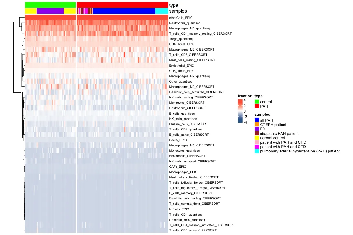
10.2 complexheatmap热图
library(ComplexHeatmap)
#整合数据-挑选了三个绝对丰度的结果
data_total <- cbind(ciber_res[,-c(24:26)],epic_res[,-1],quantiseq_res[,-1])
data_total <- as.data.frame(t(data_total))
colnames(data_total) <- data_total[1,]
data_total <- dplyr::slice(data_total,-1)
head(data_total)[1:5,1:5]

# 检查数据类型是否正确转换为数值型
data_total <- data_total %>% mutate_all(as.numeric)
# 标准化-方法3
# 范围限定在-3至3
data_total <- scale(data_total)
data_total[data_total > 3] <- 3
data_total[data_total + 3 < 0] <- -3

# 也可以用circlize创建颜色映射
# 定义颜色渐变
library(circlize)
color_fun <- colorRamp2(c(-3, 0, 3), c("#336699", "white", "tomato"))

# pd$type 和 pd$samples 是注释数据怎么上色
type_colors <- c("control" = "green", "PAH" = "red")
samples_colors <- c("all PAH" = "blue", "CTEPH patient" = "orange", "FD" = "purple",
                    "idiopathic PAH patient" = "brown", "normal control" = "yellow",
                    "patient with PAH and CHD" = "pink", "patient with PAH and CTD" = "magenta",
                    "pulmonary arterial hypertension (PAH) patient" = "cyan")

columnAnno <- HeatmapAnnotation(type = pd$group,
                                samples = pd$samples,
                                col = list(type = type_colors, samples = samples_colors))

ComplexHeatmap::Heatmap(data_total,
                        na_col = "white",
                        col = color_fun,  # 添加颜色映射函数
                        show_column_names = F,
                        row_names_side = "right",
                        name = "fraction",
                        column_order = c(colnames(data_total)[c(grep("control",pd$group),
                                                                grep("PAH",pd$group))]),
                        column_split = pd$group,
                        column_title = NULL,
                        cluster_columns = F,
                        top_annotation = columnAnno,
                        heatmap_width = unit(20, "cm"),  # 调整热图宽度
                        row_dend_width = unit(1, "cm"),  # 调整聚类树宽度
                        cluster_rows = T, # 行聚类
                        row_names_gp = gpar(fontsize = 8)  # 调整行名字体大小
                        #cluster_columns = FALSE # 列聚类。
                        )
总的来说,这个R包还是挺快捷方便的~ 里面的参数需要根据自己的数据进行调整。
参考资料:
1、Pan-cancer Immunogenomic Analyses Reveal Genotype-Immunophenotype Relationships and Predictors of Response to Checkpoint Blockade. Cell Rep. 2017 Jan 3;18(1):248-262.
2、IOBR: https://mp.weixin.qq.com/s/kb22gW6bOk_WSFt39bbyug https://iobr.github.io/book/
3、TCIA (The cancer immunome atlas): https://tcia.at/tools/toolsMain
4、生信技能树: https://mp.weixin.qq.com/s/nMeDmyO4M09z7vGnYU2K-A
注:若对内容有疑惑或者有发现明确错误的朋友,请联系后台(欢迎交流)。更多内容可关注公众号:生信方舟
- END -


 4012
4012

 被折叠的 条评论
为什么被折叠?
被折叠的 条评论
为什么被折叠?
 到【灌水乐园】发言


