


一、说明
二、什么是布朗运动?
布朗运动以罗伯特·布朗的名字命名,他是第一个在通过显微镜观察悬浮在水中的花粉粒看似随机且连续的运动时对这一现象发表评论的人之一。
布朗运动的数学模型是由阿尔伯特·爱因斯坦 (Albert Einstein) 于 1905 年提出的(这一年是他奇迹般的一年,他还发表了相对论论文)。他将花粉颗粒的运动建模为不断受到水分子的轰击,导致随机运动。
三、随机游走
布朗运动的基础是随机游走。一维随机游走定义如下:
- 一维中的简单随机游走是指向前迈出一步(+d 距离)的概率为 p,向后退一步(-d 距离)的概率为 q = 1 — p
- 使用与一维情况相同的逻辑,可以很容易地将其扩展到多个维度
随机游走是马尔可夫过程的一个例子,其中未来的行为独立于过去的历史
import random
import numpy as np
import plotly.express as px

def simulate_1d_rw(nsteps=1000, p=0.5, stepsize=1):
    steps = [ 1*stepsize if random.random() < p else -1*stepsize for i in range(nsteps) ]
    y = np.cumsum(steps)
    x = list(range(len(y)))

    return x, list(y)

simulation_data = {}
nsims = 5
for i in range(nsims):
    x, y = simulate_1d_rw()
    simulation_data['x'] = x
    simulation_data['y{col}'.format(col=i)] = y

ycols = [ 'y{col}'.format(col=i) for i in range(nsims) ]
fig = px.line(simulation_data, x='x', y=ycols)
fig.show()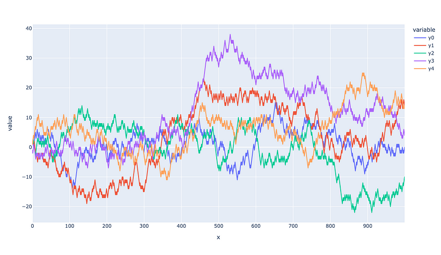
一维随机游走的多重模拟
import random
import numpy as np
import plotly.express as px

def simulate_2d(nsteps=10000, stepsize=1):

    deltas = [ (0,-1*stepsize), (-1*stepsize,0), (0,1*stepsize), (1*stepsize,0) ]

    steps = [ list(random.choice(deltas)) for i in range(nsteps) ]
    steps = np.array(steps)
    steps = np.cumsum(steps,axis=0)
    y = list(steps[:,1])
    x = list(steps[:,0])

    return x, y

x, y = simulate_2d()
fig = px.line({ 'x' : x, 'y' : y }, x='x', y='y')
fig.show()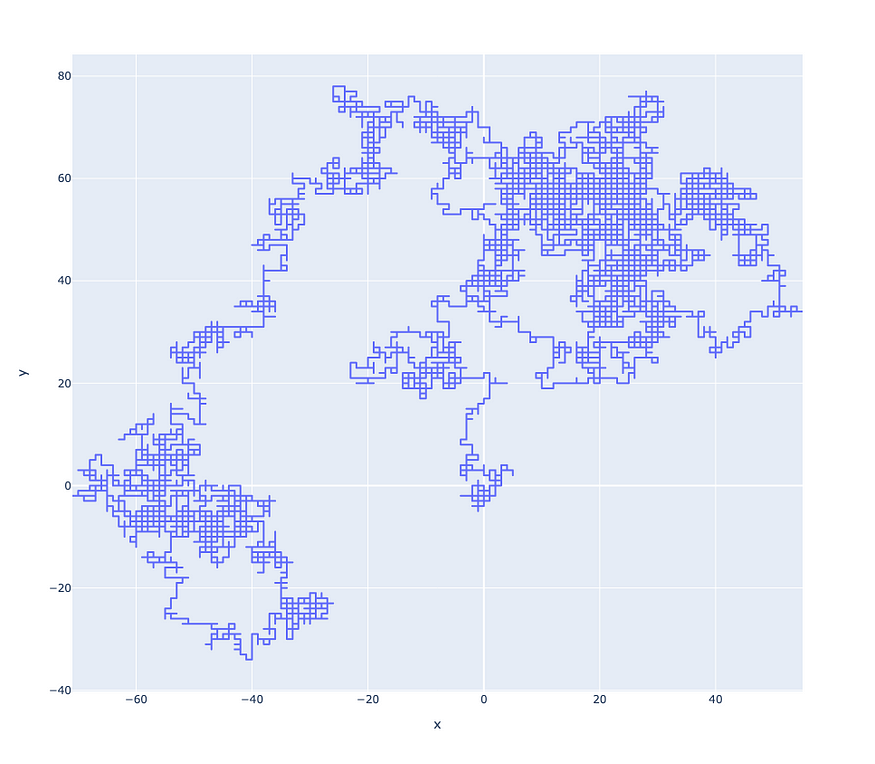
10K 步的二维随机游走模拟
import random
import numpy as np
import plotly.express as px

def simulate_3d_rw(nsteps=10000, stepsize=1):

    deltas = [ (0,0,-1*stepsize), (0,-1*stepsize,0), (-1*stepsize,0,0),\
               (0,0,1*stepsize), (0,1*stepsize,0), (1*stepsize,0,0) ]

    steps = [ list(random.choice(deltas)) for i in range(nsteps) ]
    steps = np.array(steps)
    steps = np.cumsum(steps,axis=0)
    z = list(steps[:,2])
    y = list(steps[:,1])
    x = list(steps[:,0])

    return x, y, z

x, y, z = simulate_3d_rw()
fig = px.line_3d({ 'x' : x, 'y' : y, 'z' : z }, x='x', y='y', z='z')
fig.show()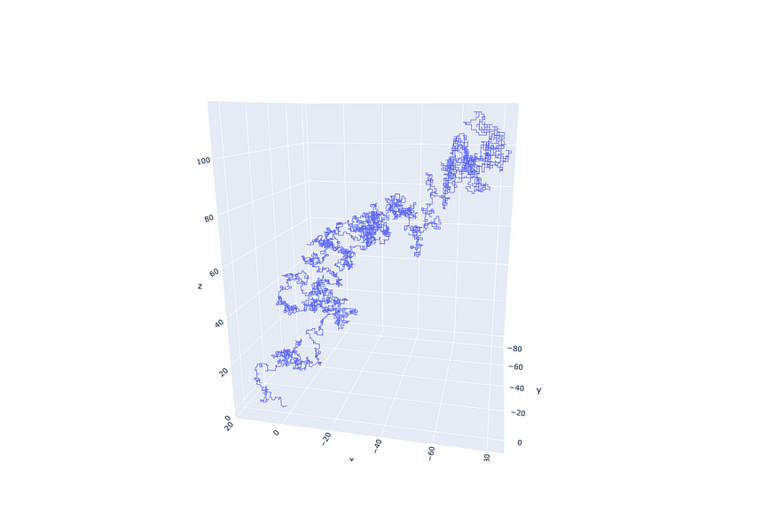
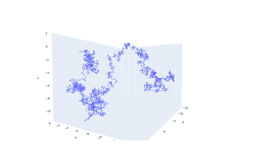
10K 步的 3-D 随机游走模拟
四、布朗运动
维纳过程是生成布朗运动的基础随机过程。维纳过程的性质如下:
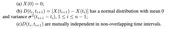
这里 X(t) 是布朗运动所经过的路径,D(t) 是布朗运动中的“步数”。通常 σ 在标准布朗运动中是常数。
当步长减小到零且时间变得连续时,布朗运动可以导出为随机游走的极限
import random
import numpy as np
import plotly.express as px

def simulate_1d_bm(nsteps=1000, t=0.01):
    steps = [ np.random.randn()*np.sqrt(t) for i in range(nsteps) ]
    y = np.cumsum(steps)
    x = [ t*i for i in range(nsteps) ]
    return x, y

nsims = 5
simulation_data = {}
for i in range(nsims):
    x, y = simulate_1d_bm()
    simulation_data['y{col}'.format(col=i)] = y
    simulation_data['x'] = x

ycols = [ 'y{col}'.format(col=i) for i in range(nsims) ]
fig = px.line(simulation_data, x='x', y=ycols)
fig.show()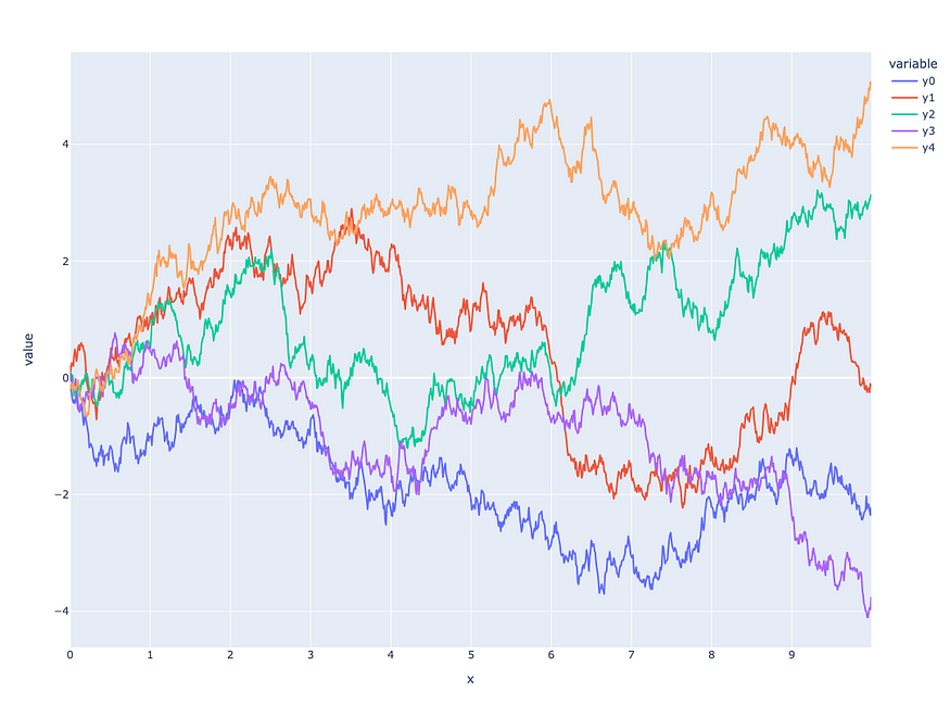
一维布朗运动的多重模拟
import random
import numpy as np
import plotly.express as px

def simulate_2d_bm(nsteps=1000, t=0.01):
    x = np.cumsum([ np.random.randn()*np.sqrt(t) for i in range(nsteps) ])
    y = np.cumsum([ np.random.randn()*np.sqrt(t) for i in range(nsteps) ])
    return list(x), list(y)

x, y = simulate_2d_bm()
fig = px.line({ 'x' : x, 'y' : y }, x='x', y='y')
fig.show()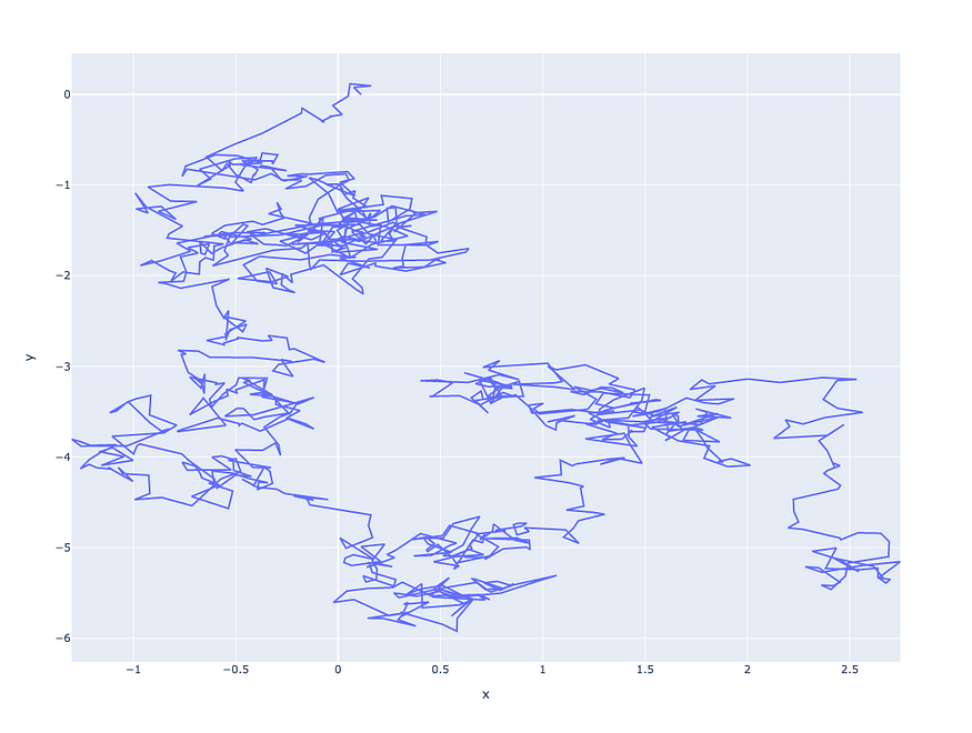
二维布朗运动的模拟
import random
import numpy as np
import plotly.express as px

def simulate_3d_bm(nsteps=10000, t=0.01):
    x = np.cumsum([ np.random.randn()*np.sqrt(t) for i in range(nsteps) ])
    y = np.cumsum([ np.random.randn()*np.sqrt(t) for i in range(nsteps) ])
    z = np.cumsum([ np.random.randn()*np.sqrt(t) for i in range(nsteps) ])
    return list(x), list(y), list(z)

x, y, z = simulate_3d_bm()
fig = px.line_3d({ 'x' : x, 'y' : y, 'z' : z }, x='x', y='y', z='z')
fig.show()
10K 步的 3-D 布朗运动模拟
4.1 带有漂移的布朗运动
这是布朗运动的变体,其中存在漂移分量以及通常的随机分量。
![]()
与带有随机噪声的 X(t) 一起是 μ*t,它是漂移
import random
import numpy as np
import plotly.express as px

def simulate_1d_bm_with_drift(nsteps=1000, t=0.01, mu=0.5):
    steps = [ mu*0.01 + np.random.randn()*np.sqrt(t) for i in range(nsteps) ]
    y = np.cumsum(steps)
    x = [ t*i for i in range(nsteps) ]
    return x, y

nsims = 5
simulation_data = {}
for i in range(nsims):
    x, y = simulate_1d_bm_with_drift()
    simulation_data['y{col}'.format(col=i)] = y
    simulation_data['x'] = x

ycols = [ 'y{col}'.format(col=i) for i in range(nsims) ]
fig = px.line(simulation_data, x='x', y=ycols)
fig.show()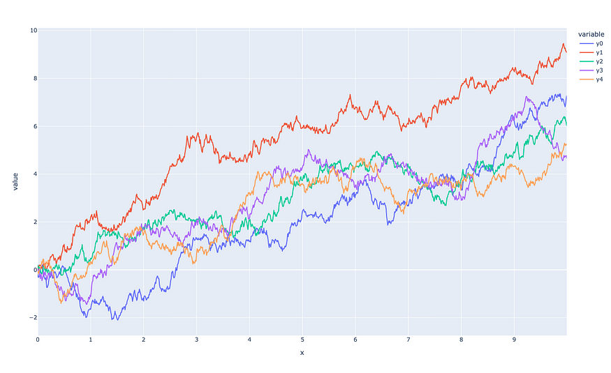
带漂移的一维布朗运动的多重模拟
五、几何布朗运动
此过程通常用于对金融股票价格或人口增长进行建模,或用于测量值不能为负的其他情况。在金融领域,它构成了布莱克-斯科尔斯方程的基础,其中对股票价格的对数回报进行了建模:主要兴趣在于衍生品的期权定价。
它的定义如下:
![]()
G(t) 不是布朗运动,但 log[G(t)] 是
![]()
import random
import numpy as np
import plotly.express as px

def simulate_1d_gbm(nsteps=1000, t=1, mu=0.0001, sigma=0.02):
    steps = [ (mu - (sigma**2)/2) + np.random.randn()*sigma for i in range(nsteps) ]
    y = np.exp(np.cumsum(steps))
    x = [ t*i for i in range(nsteps) ]
    return x, y

nsims = 5
simulation_data = {}
for i in range(nsims):
    x, y = simulate_1d_gbm()
    simulation_data['y{col}'.format(col=i)] = y
    simulation_data['x'] = x

ycols = [ 'y{col}'.format(col=i) for i in range(nsims) ]
fig = px.line(simulation_data, x='x', y=ycols)
fig.show()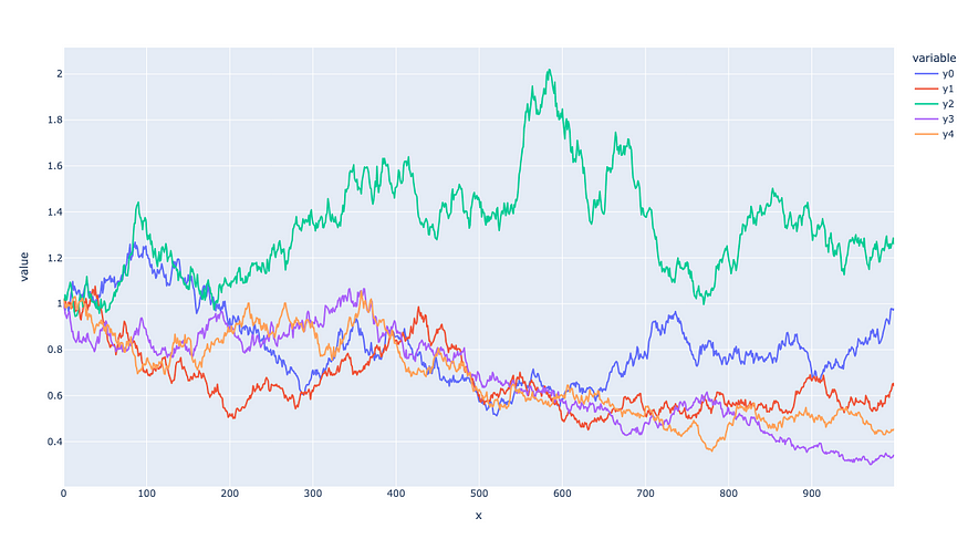
几何布朗运动的多重模拟
5.1 使用几何布朗运动模拟股票价格
从上面的定义可以看出,我们可以使用实际股票价格数据来估计μ和σ,并使用参数来模拟股票价格。在下面的示例中,我们将查看 2022-01-01 和 2022-12-31 之间(即 2022 年)的道琼斯指数。我们将估计几何布朗运动的参数,并用它来模拟股票的价格指数。
import pandas_datareader.data as web
import numpy as np
import plotly.express as px
import random

def simulate_1d_gbm(nsteps=1000, t=1, mu=0.0001, sigma=0.02, start=1):
    steps = [ (mu - (sigma**2)/2) + np.random.randn()*sigma for i in range(nsteps) ]
    y = start*np.exp(np.cumsum(steps))
    x = [ t*i for i in range(nsteps) ]
    return x, y

df = web.DataReader('^DJI', 'stooq')
mask = ( '2022-01-01' <= df.index ) & ( df.index <= '2022-12-31' )
df = df[mask]
prices = np.flip(df['Close'].values)

logprices = np.log(prices)
logreturns = logprices[1:] - logprices[:-1]
mu = np.mean(logreturns)
sigma = np.std(logreturns)
nsteps = logprices.shape[0]

x, y = simulate_1d_gbm(nsteps=nsteps, mu=mu, sigma=sigma, start=prices[0])

data = {}
data['x'] = x
data['Simulation'] = y
data['DowJonesIndex'] = prices

fig = px.line(data,x='x', y=['DowJonesIndex', 'Simulation'])
fig.show()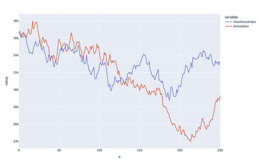
真实道琼斯指数与其模拟的比较。 x 轴是以天为单位的时间


 2954
2954

 被折叠的 条评论
为什么被折叠?
被折叠的 条评论
为什么被折叠?
 到【灌水乐园】发言


