线性拟合——从最大似然估计到平方误差到huber loss

考虑这样一些数据：

x = np.array([0,  3,  9, 14, 15, 19, 20, 21, 30, 35,
              40, 41, 42, 43, 54, 56, 67, 69, 72, 88])
                                  # x
                                  # x_i
y = np.array([33, 68, 34, 34, 37, 71, 37, 44, 48, 49,
              53, 49, 50, 48, 56, 60, 61, 63, 44, 71])
                                  # y
                                  # y_i
e = np.array([3.6, 3.9, 2.6, 3.4, 3.8, 3.8, 2.2, 2.1, 2.3, 3.8,
              2.2, 2.8, 3.9, 3.1, 3.4, 2.6, 3.4, 3.7, 2.0, 3.5])
                                  # e
                                  # e_i

作如下的可视化：

plt.errorbar(x, y, e, fmt='ok', ecolor='gray', alpha=.4)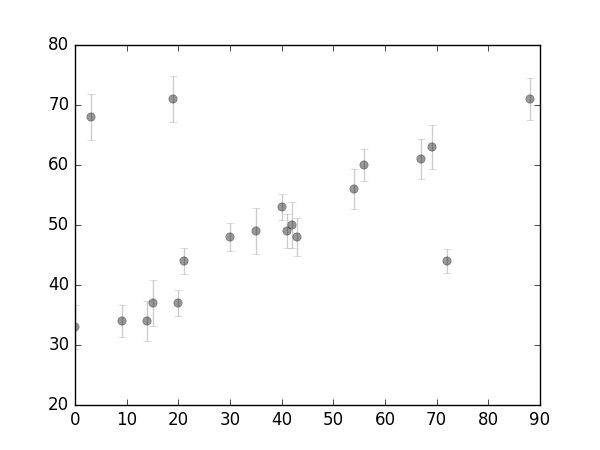

上图可见数据中存在一些离群点（outliers）。

作如下的简单建模（linear model）：

$$\hat{y}(x|\theta)=\theta_0+\theta_1x$$
在这一模型下（Given this model），我们可以分别对每一个点计算高斯型似然（Gaussian Likelihood）：
$$p(x_i,y_i,e_i|\theta)\propto\exp(-\frac1{2e_i^2}(y_i-\hat{y}(x_i|\theta))^2)$$

则全体样本$\mathcal{D}$的对数似然为：

$$\log\mathcal{L}(\mathcal{D}|\theta)=\textrm{const}-\sum_{i=1}^n\frac1{2e_i^2}(y_i-\hat{y}(x_i|\theta))^2$$
所谓最大似然，即是maximum 这一对数似然值，已获得相关参数。从优化的观点看，最大化该似然函数，等价于最小化和式项（summation term），该项被称为损失函数：
$$\mathcal{L}=\sum_{i=1}^n\frac1{2e_i^2}(y_i-\hat{y}(x_i|\theta))^2$$

该表达式即是著名的平方误差（squared loss），也即我们从高斯对数似然（Gaussian Log Likelihood）推导出了经典的平方误差（Squared Loss）的形式。

接下来我们使用两种方式进行目标函数的求解：

法一：使用scipy的最优化工具箱optimize：

from scipy import optimize

def squared_loss(theta, x=x, y=y, e=e):
    dy = (y-(theta[0]+theta[1]*x))/e
    return np.sum(dy**2/2)

theta = optimize.fmin(squared_loss, [0, 0], disp=False)

print('theta: ', theta)
                    # theta: [ 39.69978468   0.23621066]

plt.figsize(figsize=(6, 4.5))

plt.errorbar(x, y, e, fmt='ok', ecolor='gray', alpha=.4)

xfit = np.linspace(0, 100)
plt.plot(xfit, theta[0]+theta[1]*fit, -k)
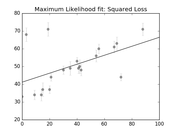
plt.title('Maximum Likelihood fit: Squared Loss')

plt.savefig('./imgs/linear_fit1.png')
plt.show()

最终得到的$\theta$：theta: [ 39.69978468 0.23621066]

法二：使用矩阵运算

为了后续矩阵运算的方便，我们首先需要对输入样本矩阵（这里为一维）做一次增广（augmentation）：

x_aug = np.hstack((np.ones((len(x), 1)), x.reshape((-1, 1))))

考虑如下的优化问题：

$$\mathcal{L}=\arg\min_{\theta}\|y-X\theta\|_2^2$$
我们可轻松地将之对 $\theta$求导（ $\frac{\partial \mathcal{L}}{\partial \theta}=0$）置零求解，以获得 $\theta$的解析解（analytical solution，或者叫closed-form solution）：
$$2X^T(X\theta-y)=0\\\theta=(X^TX)^{-1}X^Ty\\\theta=X^\dagger y$$

p_inv = np.dot(np.linalg.inv(np.dot(x_aug.T, x_aug)), x_aug.T)
theta = np.dot(p_inv, y)
print('theta:', theta)

可视化的代码一如上例，显示如下：

最终得到的 $\theta$为，theta [ 41.16631145 0.25294549]

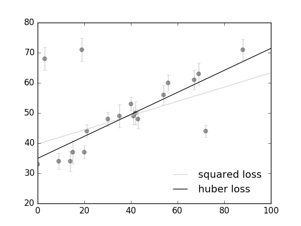
从squared loss到huber loss

从前面的可视化的拟合直线可以看出：通过最小化平方误差得到的拟合直线对离群点具有较高的敏感性，Huber loss is less sensitive to outliers in data than the squared error loss.

$$L_\delta(y,f(x))=\left\{ \begin{array}{ll} \frac12(y-f(x))^2,&\textrm{for }|y-f(x)|\leq\delta\\ \delta\cdot(|y-f(x)|-\delta/2),& \textrm{otherwise.} \end{array} \right.$$

def huber_loss(res, delta):
    return (abs(res)<delta)*res**2/2 + (abs(res)>delta)*delta(abs(res)-delta/2)

def total_huber_loss(theta, x=x, y=y, e=e, delta=3):
    return huber_loss((y-(theta[0]+theta[1]*x))/e, delta).sum()

theta1 = optimize.fmin(total_huber_loss, [0, 0], disp=False)
...