【智能算法】人工水母搜索算法（JS)原理及实现

---

1.背景

2020年，Chou 等人受到水母运动行为启发，提出了人工水母搜索算法(Artificial Jellyfish Search Optimizer, JS)。

2.算法原理

2.1算法思想

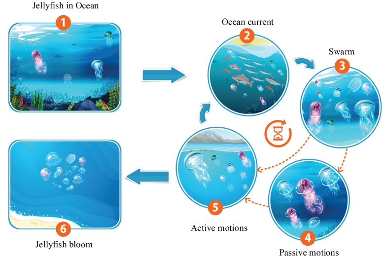
JS模拟了水母的搜索行为，包括追随海流、水母群内的主动和被动运动、时间控制机制以及群聚过程。

2.2算法过程

洋流：
海洋中蕴含着大量的营养物质，这些物质会吸引水母。洋流的方向是通过对每个水母到处于最佳位置的水母（适应度度量）所有向量进行平均。
$$\overrightarrow{\mathrm{trend}}=\frac{1}{{\mathrm{n}}_{\mathrm{Pop}}}\sum {\overrightarrow{\mathrm{trend}}}_{\mathrm{i}}=\frac{1}{{\mathrm{n}}_{\mathrm{Pop}}}\sum \left(X^{\ast }-{\mathrm{e}}_{\mathrm{c}}{X}_{\mathrm{i}}\right)=X^{\ast }-{\mathrm{e}}_{\mathrm{c}}\frac{\sum X_{\mathrm{i}}}{{\mathrm{n}}_{\mathrm{Pop}}}=X^{\ast }-{\mathrm{e}}_{\mathrm{c}}\mu$$
这里，令$\mathbf{df}={\mathbf{e}}_{\mathbf{c}}\mu$，则洋流方向可以描述为：
$$\overrightarrow{\mathrm{trend}}={\mathrm{X}}^{\ast }-\mathrm{df}$$
假设水母在所有维度上分布服从正态空间分布：

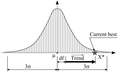
因此，可以进行简化：
$$\mathrm{df}=\beta \times \mathrm{rand}(0,1)\times \mu$$
每只水母位置更新：
$${\mathrm{X}}_{\mathrm{i}}(\mathrm{t}+1)={\mathrm{X}}_{\mathrm{i}}(\mathrm{t})+\mathrm{rand}(0,1)\times ({\mathrm{X}}^{\ast }-\beta \times \mathrm{rand}(0,1)\times \mu$$
水母群体运动：
在群集中，水母分别表现出被动（类型A）和主动（类型B）的运动 。最初，当群集刚形成时，大多数水母表现出类型A的运动。随着时间的推移，它们逐渐表现出类型B的运动。类型A运动是水母围绕自身位置的运动（全局探索），每个水母的相应更新位置由:
$${\mathrm{X}}_{\mathrm{i}}(\mathrm{t}+1)={\mathrm{X}}_{\mathrm{i}}(\mathrm{t})+\gamma \times \mathrm{rand}(0,1)\times ({\mathrm{U}}_{\mathrm{b}}-{\mathrm{L}}_{\mathrm{b}})$$
B类型运动可以看作种群间根据食物数量（适应度衡量）进行互相迁移，比如当水母$i$处食物数量大于水母$j$处，则水母$j$向水母$i$移动，反之亦然。（此阶段为局部探索）
$$\begin{gathered} \mathrm{Step}={\mathrm{X}}_{\mathrm{i}}(\mathrm{t}+1)-{\mathrm{X}}_{\mathrm{i}}(\mathrm{t}) \\ \overrightarrow{\text{Direction}}=\begin{array}{c}{\mathsf{X}}_{\mathsf{j}}(\mathsf{t})-{\mathsf{X}}_{\mathsf{i}}(\mathsf{t})\mathsf{if}\mathsf{f}({\mathsf{X}}_{\mathsf{i}})\ge \mathsf{f}({\mathsf{X}}_{\mathsf{j}})\\ {\mathsf{X}}_{\mathsf{i}}(\mathsf{t})-{\mathsf{X}}_{\mathsf{j}}(\mathsf{t})\mathsf{if}\mathsf{f}({\mathsf{X}}_{\mathsf{i}})<\mathsf{f}({\mathsf{X}}_{\mathsf{j}})\end{array} \end{gathered}$$
其中，$\overrightarrow{\mathrm{Step}}=\mathrm{rand}(0,1)\times \overrightarrow{\mathrm{Direction}}$，因此整体可表述为：
$${\mathrm{X}}_{\mathrm{i}}(\mathrm{t}+1)={\mathrm{X}}_{\mathrm{i}}(\mathrm{t})+\overrightarrow{\mathrm{Step}}$$
时间控制机制：
海洋流富含营养食物，吸引了水母的聚集形成水母群。随着温度或风向变化，水母群会转移至新的海洋流形成新的群体。水母群内的水母表现出被动和主动两种运动，其偏好会随着时间变化。引入时间控制机制来调节水母在海洋流和群内移动之间的转换。（这里是对全局与局部平衡，收敛性考虑）

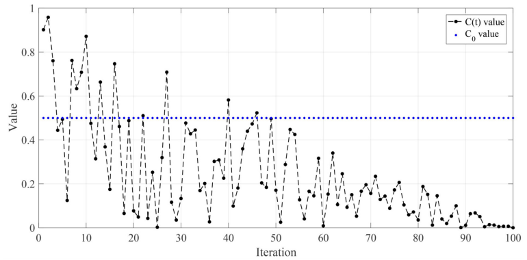
$$\mathbf{c}(\mathbf{t})=\left|\left(1-\frac{\mathbf{t}}{{\mathbf{Max}}_{\mathrm{iter}}}\right)\times (2\times \mathrm{rand}(0,1)-1)\right|$$
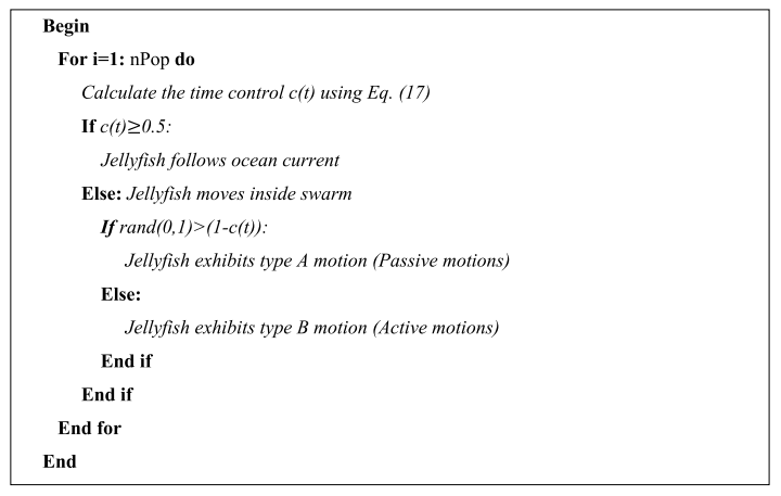
伪代码：

3.代码实现

% 水母搜索算法
function [Best_pos, Best_fitness, Iter_curve, History_pos, History_best] = JS(pop, maxIter,lb,ub,dim,fobj)
%input
%pop 种群数量
%dim 问题维数
%ub 变量上边界
%lb 变量下边界
%fobj 适应度函数
%maxIter 最大迭代次数
%output
%Best_pos 最优位置
%Best_fitness 最优适应度值
%Iter_curve 每代最优适应度值
%History_pos 每代种群位置
%History_best 每代最优个体位置
%% 初始化种群
X = initialization(pop,dim,ub,lb);
VarSize = [1 dim];
%% 计算适应度
popCost = zeros(1,pop);
for i=1:pop
    popCost(i) = fobj(X(i,:));
end
%% 迭代
for it=1:maxIter
    Meanvl=mean(X,1);
    [value,index]=sort(popCost);
    Best_pos=X(index(1),:);
    BestCost=popCost(index(1));
    for i=1:pop
        % Calculate time control c(t) using Eq. (17);
        Ar=(1-it*((1)/maxIter))*(2*rand-1);
        if abs(Ar)>=0.5
            %% Folowing to ocean current using Eq. (11)
            newsol = X(i,:)+ rand(VarSize).*(Best_pos - 3*rand*Meanvl);
            % Check the boundary using Eq. (19)
            newsol = simplebounds(newsol,lb,ub);
            % Evaluation
            newsolCost = fobj(newsol);
            % Comparison
            if newsolCost<popCost(i)
                X(i,:) = newsol;
                popCost(i)=newsolCost;
                if popCost(i) < BestCost
                    BestCost=popCost(i);
                    Best_pos = X(i,:);
                end
            end
        else
            %% Moving inside swarm
            if rand<=(1-Ar)
                % Determine direction of jellyfish by Eq. (15)
                j=i;
                while j==i
                    j=randperm(pop,1);
                end
                Step = X(i,:) - X(j,:);
                if popCost(j) < popCost(i)
                    Step = -Step;
                end
                % Active motions (Type B) using Eq. (16)
                newsol = X(i,:) + rand(VarSize).*Step;
            else
                % Passive motions (Type A) using Eq. (12)
                newsol = X(i,:) + 0.1*(ub-lb)*rand;
            end
            % Check the boundary using Eq. (19)
            newsol = simplebounds(newsol, lb,ub);
            % Evaluation
            newsolCost = fobj(newsol);
            % Comparison
            if newsolCost<popCost(i)
                X(i,:) = newsol;
                popCost(i)=newsolCost;
                if popCost(i) < BestCost
                    BestCost=popCost(i);
                    Best_pos = X(i,:);
                end
            end
        end
    end
    %% Store Record for Current Iteration
    Iter_curve(it)=BestCost;
    Best_fitness = BestCost;
    History_best{it} = Best_pos;
    History_pos{it} = X;
end
end
%% This function is for checking boundary by using Eq. 19
function s=simplebounds(s,Lb,Ub)
ns_tmp=s;
I=ns_tmp<Lb;
% Apply to the lower bound
while sum(I)~=0
    ns_tmp(I)=Ub(I)+(ns_tmp(I)-Lb(I));
    I=ns_tmp<Lb;
end
% Apply to the upper bound
J=ns_tmp>Ub;
while sum(J)~=0
    ns_tmp(J)=Lb(J)+(ns_tmp(J)-Ub(J));
    J=ns_tmp>Ub;
end
% Check results
s=ns_tmp;
end
%%
function pop=initialization(num_pop,nd,Ub,Lb)

if size(Lb,2)==1
    Lb=Lb*ones(1,nd);
    Ub=Ub*ones(1,nd);
end
x(1,:)=rand(1,nd);
a=4;
for i=1:(num_pop-1)
    x(i+1,:)=a*x(i,:).*(1-x(i,:));
end 
for k=1:nd
    for i=1:num_pop
        pop(i,k)=Lb(k)+x(i,k)*(Ub(k)-Lb(k));
    end
end
end

4.参考文献

[1] Chou J S, Truong D N. A novel metaheuristic optimizer inspired by behavior of jellyfish in ocean[J]. Applied Mathematics and Computation, 2021, 389: 125535.