[Nature AI论文]未测量流域 ungauged watersheds极端洪水的全球预测

未测量流域极端洪水的全球预测

• 灰色接近，
• 黛博拉·科恩,
• 乌苏穆兹·杜贝
• 马丁·高赫,
• 奥伦·吉隆,

• 指标细节

抽象的

洪水是最常见的自然灾害之一，对经常缺乏密集水流测量网络的发展中国家造成的影响尤为严重1。准确及时的预警对于减轻洪水风险至关重要2，但水文模拟模型通常必须根据每个流域的长数据记录进行校准。在这里，我们表明，基于人工智能的预测在预测未测量流域的极端河流事件方面实现了长达五天的可靠性，这与当前状态的临近预报（零日提前时间）的可靠性相似或更好最先进的全球建模系统（哥白尼应急管理服务全球洪水意识系统）。此外，我们在五年重现期事件中实现的精度与当前一年重现期事件的精度相似或更好。这意味着人工智能可以针对未测量流域中规模更大、影响力更大的事件更早地提供洪水预警。这里开发的模型被纳入一个可操作的早期预警系统中，该系统可在 80 多个国家实时生成公开可用（免费且开放）的预报。这项工作强调需要增加水文数据的可用性，以继续改善全球获得可靠洪水预警的机会。

其他人正在查看类似内容

利用气候和流域信息对欧洲洪水概率进行季节性预测

文章 开放获取2022 年 8 月 6 日

人工智能对气候影响：在洪水风险中的应用

文章 开放获取2023 年 6 月 8 日

从干旱灾害转向影响预测

文章 开放获取2019 年 10 月 30 日

主要的

洪水是最常见的自然灾害3，自 2000 年以来，与洪水相关的灾害发生率增加了一倍多4。与洪水相关的灾害的增加是由人为气候变化引起的水文循环加速推动的5 , 6。预警系统是减轻洪水风险的有效方法，可将洪水相关死亡人数减少高达 43% 7 , 8，并将经济成本减少 35-50% 9 , 10。在易受洪水风险影响的 18 亿人口中，中低收入国家的人口几乎占 90% 1。世界银行估计，将发展中国家的洪水预警系统升级到发达国家的标准，平均每年可挽救 23,000 人的生命2。

在本文中，我们评估了在开放公共数据集上训练的人工智能（AI）在多大程度上可用于改善全球河流极端事件预报的获取。根据本文所述的模型和实验，我们开发了一个操作系统，可以对 80 多个国家/地区进行短期（7 天）洪水预报。这些预测是实时提供的，没有任何访问障碍，例如费用或网站注册 ( https://g.co/floodhub )。

河流预报的一个主要挑战是水文预测模型必须使用长数据记录11、12 来针对各个流域进行校准。缺乏流量计来提供校准数据的流域被称为未计量流域，而“未计量流域的预测”（PUB）问题是国际水文科学协会（IAHS）从2003年到2012年的十年问题13。在 PUB 十年结束时，IAHS 报告说，在解决这个问题方面几乎没有取得任何进展，并指出“迄今为止，大部分成功都是在计量盆地而不是未计量盆地中取得的，这尤其对发展中国家产生了负面影响” 14 .

世界上只有百分之几的流域进行了测量，而且流量计在世界各地的分布并不均匀。特定国家的国内生产总值与公开可用的水流观测数据记录总量之间存在很强的相关性（扩展数据图1显示了这种双对数相关性），这意味着在以下领域进行高质量预测尤其具有挑战性：最容易受到人类洪水影响。

在之前的工作15中，我们表明机器学习可用于开发可转移到未计量流域的水文模拟模型。在这里，我们将其开发为全球规模的预测系统，目标是了解可扩展性和可靠性。在本文中，我们讨论了鉴于公开的全球水流数据记录，是否有可能提供大范围内的准确河流预测，特别是极端事件的预测，以及这与当前技术水平的比较。

目前最先进的实时全球规模水文预测是全球洪水意识系统 (GloFAS) 16 , 17。 GloFAS 是哥白尼应急管理服务 (CEMS) 的全球洪水预报系统，由欧盟委员会联合研究中心负责交付，并由欧洲中期天气预报中心 (ECMWF) 作为 CEMS 水文预报中心运营– 计算。我们使用 GloFAS 版本 4，这是 2023 年 7 月上线的当前运行版本。世界不同地区还存在其他预报系统18 , 19 , 20，许多国家都有负责产生预警的国家机构。鉴于洪水对世界各地社区影响的严重性，我们认为预测机构对其预测、预警和方法进行评估和基准测试至关重要，而实现这一目标的重要第一步是将历史预测存档。

人工智能提高预测可靠性

本研究开发的人工智能模型使用长短期记忆 (LSTM) 网络21来预测 7 天预测范围内的每日水流。该模型在方法中详细描述，并且适合研究的模型版本在开源 NeuralHydrology 存储库22中实现。输入、目标和评估数据在方法中描述。

该 AI 预测模型使用5,680 个流量计的随机k倍交叉验证进行了样本外训练和测试。方法中报告了其他类型的交叉验证实验（即，保留终端流域、整个气候区或整个大陆的所有仪表）。此外，AI 模型报告的所有指标都是使用训练中未出现的时间段的流量计数据计算的（除了训练中未出现的流量计之外），这意味着交叉验证分割在样本外时间和地点。相比之下，GloFAS 的指标是通过测量和未测量位置的组合以及校准和验证时间段的组合来计算的。这意味着比较有利于 GloFAS 基准。这是必要的，因为校准 GloFAS 的计算成本很高，以至于在交叉验证分割上重新校准是不可行的。

我们的目标是了解极端事件预测的可靠性，因此我们报告不同重现期事件的精确度、召回率和 F1 分数（F1 分数是精确度和召回率的调和平均值）。其他标准水文指标在方法中报告。统计检验在方法中描述。

图1显示了 1984 年至 2021 年期间 0 天提前期的 2 年重现期事件的 F1 分数差异的全球分布（N  = 3,360）。前置时间表示为从预测时间算起的天数，因此 0 天前置时间意味着流量预测是针对当天的（临近预报）。 AI 模型在重现期事件的 64% (65%)、70% (73%)、60% (73%) 和 49% (76%) 指标上比 GloFAS 版本 4 有所改进（至少相当于） 1 年（N  = 3,638，P  = 6 × 10 −87，科恩d  = 0.22），2 年（N  = 3,673，P  < 3 × 10 −181，d  = 0.41），5 年（N  = 3,360，P  = 8 × 10 −130 , d  = 0.42) 和 10 年 ( N  = 2,920, P  < 1 × 10 −66 , d  = 0.33)。

图 1：1984 年至 2021 年期间，我们的 AI 模型和 GloFAS 之间的 2 年重现期事件的临近预报（0 天提前期）F1 分数之间的差异。

AI 模型在 70% 的仪表中比 GloFAS 有所改进 ( N  = 3,673)。 GloFAS 模拟数据来自气候数据存储33。来自 GeoPandas 34的底图。

全尺寸图像

退货期

更极端的水文事件（即重现期较长的事件）既更重要，而且（使用经典水文模型时）通常更难以预测。关于使用人工智能或其他类型的数据驱动方法的一个常见担忧23,24,25,26是可靠性可能会因训练数据中罕见的事件而降低。先前的证据表明，这种担忧对于水流建模可能无效27。

图2显示了不同重现期事件的精确率和召回率的分布。 AI 模型在所有重现期（N  > 3,000，P  < 1 × 10 −5）都具有更高的精确度和召回率分数，效应大小范围从d  = 0.15（1 年精确度分数）到d  = 0.46（2 年精确度分数）回忆分数）。在α  = 1%（N  = 3,465，P  = 0.02，d  = -0.01）和召回率时，AI 模型在 5 年重现期事件中的精确度分数与 GloFAS 在 1 年重现期事件中的精确度分数之间的差异并不显着。 5 年事件的 AI 模型得分优于 1 年事件的 GloFAS 回忆得分（N  = 3,586，P  = 1 × 10 −18，d  = 0.20）。

图 2：临近预报（0 天提前期）精度和召回率随返回周期的变化的分布。

a , b，平均而言，AI 模型在所有回报期都更可靠。 AI 模型对 5 年重现期事件的精度与 1 年重现期事件的 GloFAS 没有统计差异，而且回想起来，它比 1 年重现期事件的 GloFAS 更好。统计测试在正文中报告。方框显示分布四分位数，须线显示排除异常值的全部范围。蓝色虚线是 1 年事件中 GloFAS 得分的中位数，绘制作为参考。刻度标签指示每个箱线图的样本大小（仪表数量）；精确度得分 ( a ) 和召回率得分 ( b ) 是在稍微不同的仪表组上计算的，如果观测或模型预测中给定仪表位置处没有给定幅度的事件，导致一个模型的一个分数未定义。在所有情况下，GloFAS 和 AI 模型始终通过一组相同的仪表进行比较。 GloFAS 模拟数据来自气候数据存储33。

全尺寸图像

预测提前期

图3显示了 1 年至 10 年回报期的 7 天预测范围内交付周期的 F1 分数。与 GloFAS 即时预报（0 天提前期）相比，AI 预测在 1 年的 5 天提前期内具有更好或没有统计差异的可靠性（F1 分数）（AI 明显更好；N  = 2,415，P  = 6 × 10 −6，d  = 0.08），2 年（无统计学差异；N  = 2,162，P  = 0.98，d  = 2 × 10 −4）和 5 年（无统计学差异；N  = 1,298，P  = 0.69, d  = 0.025) 返回周期事件。

图 3：所有评估指标上 F1 分数的分布，作为不同回报期提前期的函数。

a – d，AI 模型在 1 年 ( a )、2 年 ( b )、5 年 ( c ) 和 10 年 ( d ) 回报期事件中的 F1 分数长达 5 天，在 0 天提前期的相同事件中，其在统计上优于 GloFAS，或没有统计差异。统计测试在正文中报告。方框显示分布四分位数，须线显示排除异常值的全部范围。蓝色虚线是 GloFAS 即时预报的中值分数，绘制为参考。 GloFAS 模拟数据来自气候数据存储33。

全尺寸图像

大陆

这两种模型在世界不同地区的可靠性方面存在差异。在 5 年重现期事件中，GloFAS 在得分最低的大陆（南美洲，F1 = 0.15）和得分最高的大陆（欧洲，F1 = 0.32）的平均 F1 得分之间存在 54% 的差异，这意味着，平均而言，真阳性预测的可能性是其两倍（按比例）。 AI 模型在得分最低的大陆（南美洲，F1 = 0.21）和得分最高的大陆（西南太平洋：F1 = 0.46）的平均 F1 得分之间也存在 54% 的差异，这主要是由于大幅增长西南太平洋地区相对于 GloFAS 的技能水平 ( d  = 0.68)。

图4显示了 F1 分数在各大洲和重现期的分布。 AI 模型在所有大陆和重现期中都具有较高得分 ( P  < 1 × 10 −2 , 0.10 <  d  < 0.68)，但不存在统计差异的三个例外： 非洲超过 1 年重现期事件 ( P  = 0.07，d  = 0.03）和亚洲 5 年（P  = 0.04，d  = 0.12）和 10 年（P  = 0.18，d  = 0.12）重现期事件。

图 4：不同大陆和重现期的 F1 分数分布。

a – d，AI 模型在所有大洲在 1 年 ( a )、2 年 ( b )、5 年 ( c ) 和 10 年 ( d ) 重现期事件中得分较高，但有以下三个例外：无统​​计差异：非洲超过 1 年重现期事件，亚洲超过 5 年和 10 年重现期事件。这两种模型的可靠性之间存在巨大的基于位置的差异，可以通过增加全球开放水文数据的访问来解决这一问题。统计测试在正文中报告。方框显示分布四分位数，须线显示排除异常值的全部范围。 GloFAS 模拟数据来自气候数据存储33。

全尺寸图像

预测可靠性的可预测性

在未测量的盆地中进行预测的一个挑战是，在没有地面实况数据的情况下，通常无法评估地点的可靠性。模型的理想品质是预测技能应该可以从其他可观测变量（例如地图或遥感地理和/或地球物理数据）进行预测。此外，尽管基于人工智能的预测在大多数地方提供了更好的可靠性，但并非所有地方都是如此。能够预测不同模型在哪些方面的可靠性会更高或更低，这将是有益的。

我们发现很难使用流域属性（地理、地球物理数据）来预测一个模型在哪些方面比另一个模型表现更好。扩展数据图2显示了在 HydroATLAS 属性28的子集上训练的随机森林分类器的混淆矩阵，该分类器预测 AI 模型或 GloFAS 在每个单独的流域中是否表现更好（或相似）。分类器经过分层k折交叉验证和平衡采样的训练，通常会预测 AI 模型更好（包括在 70% 的情况下 GloFAS 实际上更好）。这表明，根据可用的流域属性，很难找到关于每个模型在哪里更可取的系统模式。

然而，通过一定的技巧，可以预测单个模型在哪些方面表现良好，哪些方面表现不佳。作为示例，图5显示了随机森林分类器的混淆矩阵，该矩阵预测样本外量规（有效未计量位置）的 F1 分数是否高于或低于所有评估量规的平均值。两种模型（AI 模型和 GloFAS）具有相似的整体可预测性（GloFAS 的微平均精确度和召回率为 71%，AI 模型为 73%）。

图 5：测试预测给定模型在任何给定位置的表现是否高于或低于平均水平的能力。

a、b ，关于每个量规上 GloFAS ( a ) 和 AI 模型 ( b ) 的 F1 分数是否高于或低于同一模型在所有量规上的平均 F1 分数的样本外预测的混淆矩阵。混淆矩阵上显示的数字是微平均精度和召回率，颜色作为这些相同数字的视觉指示。c，F1 分数与 HydroATLAS 流域属性之间的相关性，这些属性在这些经过训练的分数分类器模型中具有最高的特征重要性排名。 GloFAS 模拟数据来自气候数据存储33。

全尺寸图像

这些可靠性分类器的特征重要性显示在扩展数据图3中。特征重要性是关于哪些地球物理属性决定高可靠性和低可靠性的指标（即，这些模型模拟什么样的流域效果好还是效果差）。 AI 模型最重要的特征是：流域面积、年平均潜在蒸散量 (PET)、年平均实际蒸散量 (AET) 和海拔，而 GloFAS 最重要的特征是 PET 和 AET。属性和可靠性分数之间的相关性通常较低，表明高度的非线性和/或参数交互。

AET 和 PET 是干旱度的（反）指标，水文模型通常在潮湿盆地中表现更好，因为干旱流域中出现的峰值水位线很难模拟。两种模型都存在这种效果。 AI模型与盆地大小（流域面积）的相关性更强，通常在较小的盆地中表现更好。这表明基于机器学习的水流建模可以得到改进，例如，通过对较大流域进行集中训练或微调，或者通过实施显式路由或图形模型以允许对子流域或较小的水文响应进行直接建模单位——例如，如参考文献中所述。29 .

图6显示了该随机森林技能预测器的回归（而不是分类器）版本的预测技能的全局图，其中包含103 万个 12 级 HydroBASINS 流域30。这给出了一些关于全球版本的未经衡量的人工智能预测模型预计表现良好的迹象。

图 6：全局预测技能。

该地图显示了 AI 预测模型对 103 万个 HydroBASINS 12 级流域的 2 年重现期 F1 分数的预测。来自 GeoPandas 34的底图。

全尺寸图像

结论与讨论

尽管水文模型是一个相对成熟的研究领域，但世界上最容易遭受洪水风险的地区往往缺乏可靠的预报和预警系统。利用人工智能和开放数据集，我们能够显着提高极端河流事件短期（0-7 天）预报的预期精度、召回率和提前时间。平均而言，我们将当前可用的全球临近预报（提前时间 0）的可靠性延长至 5 天，并且我们能够使用基于人工智能的预测来提高非洲的预测技能，使其与非洲的预测类似。目前在欧洲有售。

除了提供准确的预报之外，提供可操作的洪水警报的另一个挑战是及时向个人和组织传播这些警报。我们通过实时公开发布预测来支持后者，无需任何成本或访问障碍。我们提供开放访问的实时预报来支持通知，例如，通过通用警报协议并将警报推送到个人智能手机，以及通过开放的在线门户https://g.co/floodhub。本研究使用的所有重新分析和重新预测都包含在一个开源存储库中，并且用于本研究的机器学习模型的研究版本可作为 GitHub 上开源 NeuralHydrology 存储库的一部分获得22。

全球洪水预测和预警系统仍有很大改进空间。这样做对于全世界数百万人的福祉至关重要，他们的生命（和财产）可以受益于及时、可操作的洪水预警。我们认为，通过数据驱动和概念建模方法改进洪水预报的最佳方法是增加对数据的访问。训练或校准准确的水文模型以及实时更新这些模型（例如，通过数据同化31）需要水文数据。我们鼓励能够访问流数据的研究人员和组织为开源 Caravan 项目做出贡献：https://github.com/kratzert/Caravan 32。

方法

人工智能模型

本文报告的人工智能水流预测模型扩展了参考文献中的工作。35，它使用 LSTM 网络开发了水文临近预报模型，该模型根据气象输入数据序列模拟水流数据序列。在此基础上，我们开发了一种预测模型，该模型使用编码器-解码器模型，其中一个 LSTM 运行在气象（和地球物理）输入数据的历史序列（编码器 LSTM）上，另一个独立的 LSTM 运行在 7 天的数据上。预测范围与气象预报的输入（解码器 LSTM）。模型架构如图4所示。

该模型使用 365 天的后报序列长度，这意味着每个预报序列（0-7 天）都会看到前 365 天的气象输入数据以及 0-7 天预报范围内的气象预报数据。我们为编码器和解码器 LSTM 使用了 256 个单元状态的隐藏大小、线性单元状态转移网络和非线性（具有双曲正切激活函数的全连接层）隐藏状态转移网络。该模型在 50,000 个小批量上进行训练，批量大小为 256。所有输入均通过减去训练期间数据的平均值并除以标准差来标准化。

该模型在每个时间步长预测面积归一化水流流量上的单个不对称拉普拉斯分布的（时间步长相关）参数，如参考文献中所述。36 .损失函数是异方差密度函数的联合负对数似然。需要明确的是，该模型在每个时间步长和每个预测提前期预测单独的非对称拉普拉斯分布。本文报告的结果是通过对三个单独训练的编码器-解码器 LSTM 集合的预测水位线进行平均而得到的水位线计算得出的。每个单独训练的 LSTM 的水位线被视为每个时间步长和预测提前期的预测拉普拉斯分布的中值（第 50 个百分位）流量值。

使用此处描述的数据集，AI 模型需要几个小时才能在单个 NVIDIA-V100 图形处理单元上进行训练。确切的墙上时间取决于训练期间进行验证的频率。我们使用 50 个验证步骤（每 1,000 个批次），导致完整的全局模型需要 10 小时的训练时间。

输入数据

完整数据集包括来自 5,680 个流域的总共 152,259 年的模型输入和（水流）目标。保存到磁盘的数据集的总大小（包括密集数组中的缺失值）为 60 GB。

输入数据来自以下来源。

• 来自 ECMWF 综合预报系统 (IFS) 高分辨率 (HRES) 大气模型的每日汇总单级预报。变量包括：总降水量 (TP)、2 米温度 (T2M)、地表净太阳辐射 (SSR)、地表净热辐射 (STR)、降雪量 (SF) 和地表压力 (SP)。

• ECMWF ERA5-Land 再分析中的六个变量相同。

• 降水量估算来自美国国家海洋和大气管理局 (NOAA) 气候预测中心 (CPC) 全球统一的每日降水量分析。

• NASA 综合多卫星检索 GPM (IMERG) 早期运行的降水量估算。

• 来自 HydroATLAS 数据库的地质、地球物理和人为盆地属性28。

所有输入数据都是对每个测量点或预测点的上游总面积的盆地多边形进行面积加权平均。本研究中使用的5,680个评价标准的上游总面积范围为2.1 km 2至4,690,998 km 2。

没有使用水流数据作为 AI 模型的输入，因为 (1) 实时数据并非随处可用，尤其是在未测量的位置，以及 (2) 因为基准 (GloFAS) 不使用自回归输入。我们之前讨论了如何在基于人工智能的水流模型中使用近实时目标数据31。

扩展数据 图5显示了每个来源的可用数据的时间段。在训练期间，通过使用来自另一个数据源的类似变量（例如，使用 ERA5-Land 数据估算 HRES 数据）或通过使用平均值估算缺失数据，然后添加二进制标志来指示估算值，如参考文献中所述。31 .

目标和评估数据

训练和测试目标来自全球径流数据中心（GRDC）37。扩展数据图6显示了本研究中用于训练和测试的所有流量计的位置。我们从完整的公共 GRDC 数据集中删除了流域，其中 GRDC 报告的流域面积与使用 HydroBASINS 存储库中的流域多边形计算的流域面积相差 20% 以上 - 这是必要的，以确保由于流域划分不完善而导致数据质量较差，未用于训练。这给我们留下了 5,680 个仪表。自从我们进行了本文报道的实验以来，GRDC 已经为其测量仪位置发布了流域多边形，因此不再需要将测量仪与 HydroBASINS 流域边界相匹配。

实验

我们使用一组交叉验证实验评估了人工智能模型的性能。来自 5,680 个仪表的数据分为两种方式。首先，使用设计的交叉验证折叠对数据进行时间分割，以便在来自任何量具的任何测试数据的 1 年内（LSTM 编码器的序列长度）内不使用来自任何量具的训练数据。其次，使用k = 10 的随机（无替换） k倍交叉验证在空间中分割数据。 重复这对交叉验证过程，以便在一个模型中预测来自所有量具的所有数据（1984-2021）。这在时间和空间上都是样本外的。这避免了训练和测试之间任何潜在的数据泄漏。这些交叉验证实验是本文正文中报道的内容。

我们进行的其他交叉验证实验包括如上所述在时间上分割仪表数据，并根据以下协议在空间上非随机地分割仪表数据。

• 交叉验证分布在各大洲 ( k  = 6)。

• 交叉验证跨气候区划分（k  = 13）。

• 交叉验证在水文上分离的流域组之间进行分割（k  = 8），这意味着在任何交叉验证分割中，没有终端流域同时为训练和测试提供任何仪表。

这些交叉验证分割中的量规显示在扩展数据图7中。这些交叉验证分割的结果在扩展数据图中报告。8和9。

格罗FAS

GloFAS 输入与 AI 模型中使用的输入数据类似，主要区别如下。

• GloFAS 使用 ERA5 作为强制数据，而不是 ERA5-Land。

• GloFAS（在此处使用的数据集中）不使用 ECMWF IFS 作为模型的输入。 （AI 模型仅使用 IFS 数据进行预测，我们总是与 GloFAS 即时预报进行比较。）

• GloFAS 不使用 NOAA CPC 或 NASA IMERG 数据作为模型的直接输入。

GloFAS 在 3 弧分网格（大约 5 公里水平分辨率）上提供预测。为了避免GRDC提供的流域面积与GloFAS排水管网之间存在较大差异，所有流域面积小于500 km 2的GRDC站点均被丢弃。其余仪表在 GloFAS 网格上进行地理定位，并检查 GRDC 提供的排水面积与 GloFAS 排水网络之间的差异。如果流域面积之间的差异大于 10%，即使在 GloFAS 网格上手动修正站点位置后，站点也会被丢弃。在 GloFAS 网格上对总共 4,090 个 GRDC 站进行了地理定位。

此外，与 AI 模型不同，GloFAS 并未完全在样本外进行测试。 GloFAS 预测来自测量和未测量流域的组合，以及校准和验证时间段的组合。扩展数据 图6显示了 GloFAS 校准的仪表位置。这是必要的，因为与校准 GloFAS 相关的计算费用（例如，交叉验证分割）相关。有关 GloFAS 校准的更多信息可以在 GloFAS Wiki 38上找到。

这意味着与 AI 模型的比较有利于 GloFAS。扩展数据图9显示了在 GloFAS 校准位置使用一组标准水文指标的分数，并且可以与扩展数据图8进行比较，后者显示了所有评估位置中的相同指标。

尽管 CEMS 发布了 GloFAS 版本 4 的完整历史重新分析（无交付周期），但 GloFAS 版本 4 的重新预测（过去的预测）的长期存档并不跨越分析时的全年。鉴于可靠性指标必须考虑事件峰值的时间，这意味着只能在 0 天的交付时间内对 GloFAS 进行基准测试。

指标

正文中的结果报告了根据重现期定义的事件预测计算出的精确度和召回率指标。两种模型的精确度和召回率指标均按仪表单独计算。使用美国地质调查局公报 17b 39描述的方法，分别计算建模和观测时间序列上 5,680 个仪表中的每一个的重现期（分别计算观测时间序列和建模时间序列的重现期）。如果建模的水文过程线和观测到的水文过程线在两天内都超过了各自的重现期阈值流量值，我们认为模型正确预测了给定重现期的事件。每个量规的精确度、召回率和 F1 分数均以标准方式分别计算。我们强调，所有模型都是与实际的水流观测结果进行比较的，但事实并非如此，例如，通过比较 AI 模型的水文过程线与 GloFAS 的水文过程线来直接计算指标。值得注意的是，对于给定规格的给定模型，由于没有预测或没有观察到给定幅度（返回周期）的事件，精度或召回率可能是不确定的，但情况并非总是如此当召回未定义时，精度也未定义，反之亦然。这会导致例如图2中所示的精度和召回样本大小的差异。

本文报告的所有统计显着性值均使用双边 Wilcoxon（配对）符号秩检验进行评估。效应大小以 Cohen 术语d 40报告，使用以下惯例进行报告：具有更好平均预测的 AI 模型会产生正效应大小，反之亦然。所有箱线图均显示分布四分位数（即，中心条显示中位数，而不是均值），误差线涵盖整个数据范围（不包括异常值）。本文报告的所有结果并非都使用全部 5,680 个量表，因为某些量表没有足够的样本来计算某些重现期事件的精确度和召回率分数。每个结果都会注明样本量。

水文学家使用大量指标来评估水文模拟41，特别是极端事件42。其中一些标准指标在扩展数据表1中进行了描述，并在扩展数据图8中报告了本文中描述的模型，包括偏差、纳什-萨特克利夫效率 (NSE) 43和克林-古普塔效率 (KGE) 44。 KGE 是 GloFAS 校准的指标。扩展数据图9显示了相同的指标，但仅在校准了 GloFAS 的仪表上计算（AI 模型在这些仪表中仍然不在样本中）。扩展数据图中的结果。图 8和图 9显示，根据 GloFAS 校准指标 (KGE) 进行评估时，未计量 AI 模型在未计量盆地中的表现与 GloFAS 在计量盆地中的表现大致相同，并且在未计量盆地中的表现优于 GloFAS 在计量盆地中的表现。 （密切相关）NSE 指标。然而，在校准位置（尽管未校准位置），GloFAS 比未测量的 AI 模型具有更好的总体方差（Alpha-NSE 指标），这表明 AI 模型可能得到改进的潜在方法。

数据可用性

本研究的人工智能模型生成的重新分析（1984-2021）和重新预测（2014-2021）数据以及相应的 GloFAS 基准数据可在AI Increases Global Access to Reliable Flood Forecasts上获取（参考文献 1）。45）。气候数据存储33中的 GloFAS 版本 3 和 GloFAS 版本 4 均提供每日河流流量模拟。有关 GloFAS 版本控制的摘要，请参阅GloFAS versioning system - Copernicus Emergency Management Service - CEMS - ECMWF Confluence Wiki。

代码可用性

可以在https://doi.org/10.5281/zenodo.10397664（参考文献45 ）找到功能齐全的训练模型。这些训练好的模型是可以运行的，但我们缺乏输入数据产品的分发许可，因此要运行它们，您必须自己获取并预处理相关的输入数据。输入数据可以从以下来源获得：NASA IMERG 降水数据，Data | NASA Global Precipitation Measurement Mission； ECMWF HRES 预测数据，Atmospheric Model high resolution 10-day forecast | ECMWF； ECMWF ERA5-Land 数据，https://cds.climate.copernicus.eu/cdsapp#!/ dataset/reanalysis-era5-land?tab=overview ； NOAA CPC 全球统一日降水量数据分析，: NOAA Physical Sciences Laboratory。此外，为该项目开发的预测模型（以及其他几个 AI 水流预测模型）已集成到 NeuralHydrology 代码库22中，该代码库可在https://neuralHydrology.github.io上找到。在 NeuralHydrology 框架中使用这些研究级模型可以更轻松地使用您自己的输入数据集运行概念上相似的模型。用于重现本文报告的数据和分析的代码可在GitHub - google-research-datasets/global_streamflow_model_paper上找到。如本文所述，该存储库计算 AI 模型和 GloFAS 输出的指标，并需要 Zenodo 数据集45。

参考

1. Rentschler, J.、Salhab, M. 和 Jafino, BA 188 个国家的洪水风险和贫困。纳特。交流。 13、3527 (2022)。

   文章 中科院 考研 考研中心 谷歌学术 

2. Hallegatte, S.减少发展中国家灾害损失的成本有效解决方案：水文气象服务、预警和疏散政策研究工作文件 6058（世界银行，2012 年）。

3. 自然灾害的人类成本：全球视角（联合国国际减灾战略，2015 年）。

4. 2021 年气候服务状况WMO-No. 1278（世界气象组织，2021）。

5. Milly, P.、Christopher, D.、Wetherald, RT、Dunne, KA 和 Delworth, TL 在气候变化的情况下，大洪水的风险不断增加。自然 415 , 514–517 (2002)。

   文章 中科院 考研 谷歌学术 

6. Tabari, H. 气候变化对洪水和极端降水的影响随着可用水量的增加而增加。科学。报告 10 , 13768 (2020)。

   文章 中科院 考研 考研中心 谷歌学术 

Global prediction of extreme floods in ungauged watersheds

• Grey Nearing, 
• Deborah Cohen, 

Abstract

Floods are one of the most common natural disasters, with a disproportionate impact in developing countries that often lack dense streamflow gauge networks1. Accurate and timely warnings are critical for mitigating flood risks2, but hydrological simulation models typically must be calibrated to long data records in each watershed. Here we show that artificial intelligence-based forecasting achieves reliability in predicting extreme riverine events in ungauged watersheds at up to a five-day lead time that is similar to or better than the reliability of nowcasts (zero-day lead time) from a current state-of-the-art global modelling system (the Copernicus Emergency Management Service Global Flood Awareness System). In addition, we achieve accuracies over five-year return period events that are similar to or better than current accuracies over one-year return period events. This means that artificial intelligence can provide flood warnings earlier and over larger and more impactful events in ungauged basins. The model developed here was incorporated into an operational early warning system that produces publicly available (free and open) forecasts in real time in over 80 countries. This work highlights a need for increasing the availability of hydrological data to continue to improve global access to reliable flood warnings.

Similar content being viewed by others

Towards seasonal forecasting of flood probabilities in Europe using climate and catchment information

Article Open access06 August 2022

AI for climate impacts: applications in flood risk

Article Open access08 June 2023

Moving from drought hazard to impact forecasts

Article Open access30 October 2019

Main

Floods are the most common type of natural disaster3 and the rate of flood-related disasters has more than doubled since 20004. This increase in flood-related disasters is driven by an accelerating hydrological cycle caused by anthropogenic climate change5,6. Early warning systems are an effective way to mitigate flood risks, reducing flood-related fatalities by up to 43%7,8 and economic costs by 35–50%9,10. Populations in low- and middle-income countries make up almost 90% of the 1.8 billion people that are vulnerable to flood risks1. The World Bank has estimated that upgrading flood early warning systems in developing countries to the standards of developed countries would save an average of 23,000 lives per year2.

In this paper, we evaluate the extent to which artificial intelligence (AI) trained on open, public datasets can be used to improve global access to forecasts of extreme events in global rivers. On the basis of the model and experiments described in this paper, we developed an operational system that produces short-term (7-day) flood forecasts in over 80 countries. These forecasts are available in real time without barriers to access such as monetary charge or website registration (https://g.co/floodhub).

A major challenge for riverine forecasting is that hydrological prediction models must be calibrated to individual watersheds using long data records11,12. Watersheds that lack stream gauges to supply data for calibration are called ungauged basins, and the problem of ‘prediction in ungauged basins’ (PUB) was the decadal problem of the International Association of Hydrological Sciences (IAHS) from 2003 to 201213. At the end of the PUB decade, the IAHS reported that little progress had been made against the problem, stating that “much of the success so far has been in gauged rather than in ungauged basins, which has negative effects in particular for developing countries”14.

Only a few per cent of the world’s watersheds are gauged, and stream gauges are not distributed uniformly across the world. There is a strong correlation between national gross domestic product and the total publicly available streamflow observation data record in a given country (Extended Data Fig. 1 shows this log–log correlation), which means that high-quality forecasts are especially challenging in areas that are most vulnerable to the human impacts of flooding.

In previous work15, we showed that machine learning can be used to develop hydrological simulation models that are transferable to ungauged basins. Here we develop that into a global-scale forecasting system with the goal of understanding scalability and reliability. In this paper, we address whether, given the publicly available global streamflow data record, it is possible to provide accurate river forecasts across large scales, especially of extreme events, and how this compares with the current state of the art.

The current state of the art for real-time, global-scale hydrological prediction is the Global Flood Awareness System (GloFAS)16,17. GloFAS is the global flood forecasting system of Copernicus Emergency Management Service (CEMS), delivered under the responsibility of the European Commission’s Joint Research Centre and operated by the European Centre for Medium-Range Weather Forecasts (ECMWF) in its role of CEMS Hydrological Forecast Centre – Computation. We use GloFAS version 4, which is the current operational version that went live in July 2023. Other forecasting systems exist for different parts of the world18,19,20, and many countries have national agencies responsible for producing early warnings. Given the severity of impacts that floods have on communities around the world, we consider it critical that forecasting agencies evaluate and benchmark their predictions, warnings and approaches, and an important first step towards this goal is archiving historical forecasts.

AI improves forecast reliability

The AI model developed for this study uses long short-term memory (LSTM) networks21 to predict daily streamflow through a 7-day forecast horizon. The model is described in detail in Methods, and a version of the model suitable for research is implemented in the open-source NeuralHydrology repository22. Input, target and evaluation data are described in Methods.

This AI forecast model was trained and tested out-of-sample using random k-fold cross-validation across 5,680 streamflow gauges. Other types of cross-validation experiment are reported in Methods (that is, by withholding all gauges in terminal watersheds, entire climate zones or entire continents). In addition, all metrics reported for the AI model were calculated with streamflow gauge data from time periods not present in training (in addition to stream gauges that were not present in training), meaning that cross-validation splits were out-of-sample across time and location. By contrast, metrics for GloFAS were calculated over a combination of gauged and ungauged locations, and over a combination of calibration and validation time periods. This means that the comparison favours the GloFAS benchmark. This is necessary because calibrating GloFAS is computationally expensive to the extent that it is not feasible to re-calibrate over cross-validation splits.

Our objective is to understand the reliability of forecasts of extreme events, so we report precision, recall and F1 scores (F1 scores are the harmonic mean of precision and recall) over different return period events. Other standard hydrological metrics are reported in Methods. Statistical tests are described in Methods.

Figure 1 shows the global distribution of F1 score differences for 2-year return period events at a 0-day lead time over the period 1984–2021 (N = 3,360). Lead time is expressed as the number of days from the time of prediction, such that a 0-day lead time means that streamflow predictions are for the current day (nowcasts). The AI model improved over (was at least equivalent to) GloFAS version 4 in 64% (65%), 70% (73%), 60% (73%) and 49% (76%) of gauges for return period events of 1 year (N = 3,638, P = 6 × 10−87, Cohen’s d = 0.22), 2 years (N = 3,673, P < 3 × 10−181, d = 0.41), 5 years (N = 3,360, P = 8 × 10−130, d = 0.42) and 10 years (N = 2,920, P < 1 × 10−66, d = 0.33).

Fig. 1: Differences between nowcast (0-day lead time) F1 scores for 2-year return period events between our AI model and GloFAS over the period 1984–2021.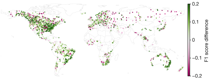

The AI model improves over GloFAS in 70% of gauges (N = 3,673). GloFAS simulation data from the Climate Data Store33. Basemap from GeoPandas34.

Full size image

Return periods

More extreme hydrological events (that is, events with larger return periods) are both more important and (when using classical hydrology models) typically more difficult to predict. A common concern23,24,25,26 about using AI or other types of data-driven approach is that reliability might degrade over events that are rare in the training data. There is prior evidence that this concern might not be valid for streamflow modelling27.

Figure 2 shows the distributions over precision and recall for different return period events. The AI model has higher precision and recall scores for all return periods (N > 3,000, P < 1 × 10−5), with effect sizes ranging from d = 0.15 (1-year precision scores) to d = 0.46 (2-year recall scores). Differences between precision scores from the AI model over 5-year return period events and from GloFAS over 1-year return period events are not significant at α = 1% (N = 3,465, P = 0.02, d = −0.01), and recall scores from the AI model for 5-year events are better than GloFAS recall scores for 1-year events (N = 3,586, P = 1 × 10−18, d = 0.20).

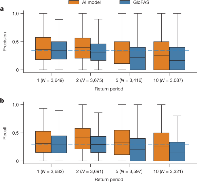
Fig. 2: Distributions over nowcast (0-day lead time) precision and recall as a function of return period.

a,b, The AI model is more reliable, on average, over all return periods. The AI model has precision over 5-year return period events that is not statistically different to GloFAS over 1-year return period events, and recall that is better than GloFAS over 1-year return period events. Statistical tests are reported in the main text. The boxes show distribution quartiles and whiskers show the full range excluding outliers. The blue dashed line is the median score for GloFAS over 1-year events and is plotted as a reference. Tick labels indicate the sample size (number of gauges) for each boxplot; precision scores (a) and recall scores (b) were calculated over slightly different gauge groups in cases where there are no events of a given magnitude at a given gauge location in either the observations or model predictions causing one score for one model to be undefined. GloFAS and the AI model are always compared over an identical set of gauges in all cases. GloFAS simulation data from the Climate Data Store33.

Full size image

Forecast lead time

Figure 3 shows F1 scores over lead times through the 7-day forecast horizon for return periods between 1 year and 10 years. Compared with GloFAS nowcasts (0-day lead time), AI forecasts have either better or not statistically different reliability (F1 scores) up to a 5-day lead time for 1-year (AI is significantly better; N = 2,415, P = 6 × 10−6, d = 0.08), 2-year (no statistical difference; N = 2,162, P = 0.98, d = 2 × 10−4) and 5-year (no statistical difference; N = 1,298, P = 0.69, d = 0.025) return period events.

Fig. 3: Distributions over F1 scores at all evaluation gauges as a function of lead time for different return periods.

a–d, The AI model has F1 scores over 1-year (a), 2-year (b), 5-year (c) and 10-year (d) return period events at up to 5-day lead times that are either statistically better than or not statistically different to GloFAS over the same events at 0-day lead time. Statistical tests are reported in the main text. The boxes show distribution quartiles and whiskers show the full range excluding outliers. The blue dashed line is the median score for GloFAS nowcasts and is plotted as a reference. GloFAS simulation data from the Climate Data Store33.

Full size image

Continents

Both models show differences in reliability in different areas of the world. Over 5-year return period events, GloFAS has a 54% difference between mean F1 scores in the lowest-scoring continent (South America, F1 = 0.15) and the highest-scoring continent (Europe, F1 = 0.32), meaning that, on average, true positive predictions are twice as likely (at a proportional rate). The AI model also has a 54% difference between mean F1 scores in the lowest-scoring continent (South America, F1 = 0.21) and the highest-scoring continent (Southwest Pacific: F1 = 0.46), which is due mostly to a large increase in skill in the Southwest Pacific relative to GloFAS (d = 0.68).

Figure 4 shows the distributions of F1 scores over continents and return periods. The AI model has higher scores in all continents and return periods (P < 1 × 10−2, 0.10 < d < 0.68) with three exceptions where there is no statistical difference: Africa over 1-year return period events (P = 0.07, d = 0.03) and Asia over 5-year (P = 0.04, d = 0.12) and 10-year (P = 0.18, d = 0.12) return period events.

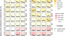
Fig. 4: F1 score distributions over different continents and return periods.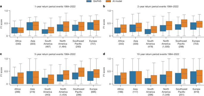

a–d, The AI model has higher scores in all continents over 1-year (a), 2-year (b), 5-year (c) and 10-year (d) return period events with three exceptions where there is no statistical difference: Africa over 1-year return period events and Asia over 5-year and 10-year return period events. Both models have large location-based differences between reliability that could be addressed by increasing global access to open hydrological data. Statistical tests are reported in the main text. The boxes show distribution quartiles and whiskers show the full range excluding outliers. GloFAS simulation data from the Climate Data Store33.

Full size image

Predictability of forecast reliability

A challenge to forecasting in ungauged basins is that there is often no way to evaluate reliability in locations without ground-truth data. A desirable quality of a model is that forecast skill should be predictable from other observable variables, such as mapped or remotely sensed geographical and/or geophysical data. In addition, although AI-based forecasting offers better reliability in most places, this is not the case everywhere. It would be beneficial to be able to predict where different models can be expected to be more or less reliable.

We have found that it is difficult to use catchment attributes (geographical, geophysical data) to predict where one model performs better than another. Extended Data Fig. 2 shows a confusion matrix from a random forest classifier trained on a subset of HydroATLAS attributes28 that predicts whether the AI model or GloFAS performs better (or similar) in each individual watershed. The classifier was trained with stratified k-fold cross-validation and balanced sampling, and usually predicts that the AI model is better (including in 70% of cases where GloFAS is actually better). This indicates that it is difficult to find systematic patterns about where each model is preferable, based on available catchment attributes.

However, it is possible to predict, with some skill, where an individual model will perform well versus poorly. As an example, Fig. 5 shows confusion matrices from random forest classifiers that predict whether F1 scores for out-of-sample gauges (effectively ungauged locations) will be above or below the mean over all evaluation gauges. Both models (the AI model and GloFAS) have similar overall predictability (71% micro-averaged precision and recall for GloFAS and 73% for the AI model).

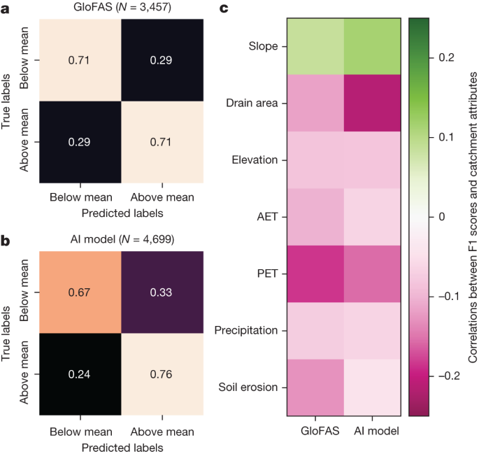
Fig. 5: Testing the ability to predict whether a given model will perform above or below average at any given location.

a,b, Confusion matrices of out-of-sample predictions about whether F1 scores from GloFAS (a) and the AI model (b) at each gauge are above or below the mean F1 score from the same model over all gauges. The numbers shown on the confusion matrices are micro-averaged precision and recall, and the colours serve as a visual indication of these same numbers. c, Correlations between F1 scores and HydroATLAS catchment attributes that have the highest feature importance ranks from these trained score classifier models. GloFAS simulation data from the Climate Data Store33.

Full size image

Feature importances from these reliability classifiers are shown in Extended Data Fig. 3. Feature importance is an indicator about which geophysical attributes determine high versus low reliability (that is, what kind of watersheds do these models simulate well versus poorly). The most important features for the AI model are: drainage area, mean annual potential evapotranspiration (PET), mean annual actual evapotranspiration (AET) and elevation, whereas the most important features for GloFAS were PET and AET. Correlations between attributes and reliability scores are generally low, indicating a high degree of nonlinearity and/or parameter interaction.

AET and PET are (inverse) indicators of aridity, and hydrology models usually perform better in humid basins because peaky hydrographs that occur in arid watersheds are difficult to simulate. This effect is present for both models. The AI model is more correlated with basin size (drainage area) and generally performs better in smaller basins. This indicates a way that machine-learning-based streamflow modelling might be improved, for example, by focusing training or fine-tuning on larger basins, or by implementing an explicit routing or graph model to allow for direct modelling of subwatersheds or smaller hydrological response units—for example, as outlined in ref. 29.

A global map of the predicted skill from a regression (rather than classifier) version of this random forest skill predictor is shown in Fig. 6 for 1.03 million level-12 HydroBASINS watersheds30. This gives some indication about where a global version of the ungauged AI forecast model is expected to perform well.

Fig. 6: Global predicted skill.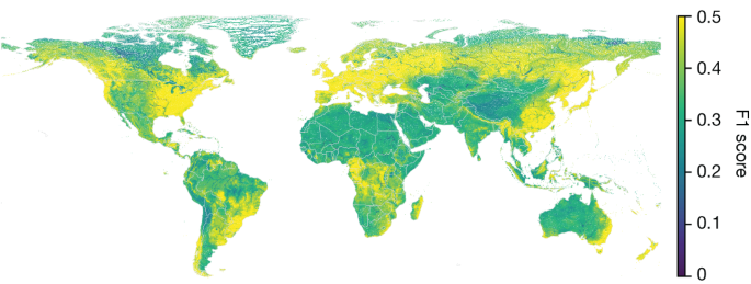

This map shows predictions of 2-year return period F1 scores over 1.03 million HydroBASINS level-12 watersheds for the AI forecast model. Basemap from GeoPandas34.

Full size image

Conclusion and discussion

Although hydrological modelling is a relatively mature area of study, areas of the world that are most vulnerable to flood risks often lack reliable forecasts and early warning systems. Using AI and open datasets, we are able to significantly improve the expected precision, recall and lead time of short-term (0–7 days) forecasts of extreme riverine events. We extended, on average, the reliability of currently available global nowcasts (lead time 0) to a lead time of 5 days, and we were able to use AI-based forecasting to improve the skill of forecasts in Africa to be similar to what are currently available in Europe.

Apart from producing accurate forecasts, another aspect of the challenge of providing actionable flood warnings is dissemination of those warnings to individuals and organizations in a timely manner. We support the latter by releasing forecasts publicly in real time, without cost or barriers to access. We provide open-access real-time forecasts to support notifications—for example, through the Common Alerting Protocol and push alerts to personal smartphones, and through an open online portal at https://g.co/floodhub. All of the reanalysis and reforecasts used for this study are included in an open-source repository, and a research version of the machine-learning model used for this study is available as part of the open-source NeuralHydrology repository on GitHub22.

There is still a lot of room to improve global flood predictions and early warning systems. Doing so is critical for the well-being of millions of people worldwide whose lives (and property) could benefit from timely, actionable flood warnings. We believe that the best way to improve flood forecasts from both data-driven and conceptual modelling approaches is to increase access to data. Hydrological data are required for training or calibrating accurate hydrology models, and for updating these models in real time (for example, through data assimilation31). We encourage researchers and organizations with access to streamflow data to contribute to the open-source Caravan project at GitHub - kratzert/Caravan: A global community dataset for large-sample hydrology32.

Methods

AI model

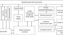
The AI streamflow forecasting model reported in this paper extends work in ref. 35, which developed hydrological nowcast models using LSTM networks that simulate sequences of streamflow data from sequences of meteorological input data. Building on that, we developed a forecast model that uses an encoder–decoder model with one LSTM running over a historical sequence of meteorological (and geophysical) input data (the encoder LSTM) and another, separate, LSTM that runs over the 7-day forecast horizon with inputs from meteorological forecasts (the decoder LSTM). The model architecture is illustrated in Extended Data Fig. 4.

The model uses a hindcast sequence length of 365 days, meaning that every forecast sequence (0–7 days) saw meteorological input data from the preceding 365 days and meteorological forecast data over the 0–7-day forecast horizon. We used a hidden size of 256 cell states for both the encoder and decoder LSTMs, a linear-cell-state transfer network and a nonlinear (fully connected layer with hyperbolic tangent activation functions) hidden-state transfer network. The model was trained on 50,000 minibatches with a batch size of 256. All inputs were standardized by subtracting the mean and dividing by the standard deviation of training-period data.

The model predicts, at each time step, (time-step dependent) parameters of a single asymmetric Laplacian distribution over area-normalized streamflow discharge, as described in ref. 36. The loss function is the joint negative log-likelihood of that heteroscedastic density function. To be clear, the model predicts a separate asymmetric Laplacian distribution at each time step and each forecast lead time. The results reported in this paper were calculated over a hydrograph that results from averaging the predicted hydrographs from an ensemble of three separately trained encoder–decoder LSTMs. The hydrograph from each of these separately trained LSTMs is taken as the median (50th percentile) flow value from the predicted Laplacian distribution at each time step and forecast lead time.

Using the dataset described herein, the AI model takes a few hours to train on a single NVIDIA-V100 graphics processing unit. The exact wall time depends on how often validation is done during training. We use 50 validation steps (every 1,000 batches), resulting in a 10-hour train time for the full global model.

Input data

The full dataset includes model inputs and (streamflow) targets for a total of 152,259 years from 5,680 watersheds. The total size of the dataset saved to disk (including missing values in a dense array) is 60 GB.

Input data came from the following sources.

• Daily-aggregated single-level forecasts from the ECMWF Integrated Forecast System (IFS) High Resolution (HRES) atmospheric model. Variables include: total precipitation (TP), 2-m temperature (T2M), surface net solar radiation (SSR), surface net thermal radiation (STR), snowfall (SF) and surface pressure (SP).

• The same six variables from the ECMWF ERA5-Land reanalysis.

• Precipitation estimates from the National Oceanic and Atmospheric Administration (NOAA) Climate Prediction Center (CPC) Global Unified Gauge-Based Analysis of Daily Precipitation.

• Precipitation estimates from the NASA Integrated Multi-satellite Retrievals for GPM (IMERG) early run.

• Geological, geophysical and anthropogenic basin attributes from the HydroATLAS database28.

All input data were area-weighted averaged over basin polygons over the total upstream area of each gauge or prediction point. The total upstream area for the 5,680 evaluation gauges used in this study ranged from 2.1 km2 to 4,690,998 km2.

No streamflow data were used as inputs to the AI model because (1) real-time data are not available everywhere, especially in ungauged locations, and (2) because the benchmark (GloFAS) does not use autoregressive inputs. We previously discussed how to use near-real-time target data in an AI-based streamflow model31.

Extended Data Fig. 5 shows the time periods of available data from each source. During training, missing data was imputed either by using a similar variable from another data source (for example, HRES data were imputed with ERA5-Land data), or by imputing with a mean value and then adding a binary flag to indicate an imputed value, as described in ref. 31.

Target and evaluation data

Training and test targets came from the Global Runoff Data Center (GRDC)37. Extended Data Fig. 6 shows the location of all streamflow gauges used in this study for both training and testing. We removed watersheds from the full, public GRDC dataset where drainage area reported by GRDC differed by more than 20% from drainage area calculated using watershed polygons from the HydroBASINS repository—this was necessary to ensure that poor-quality data, owing to imperfect catchment delineation, was not used for training. This left us with 5,680 gauges. Since we conducted the experiments reported in this paper, the GRDC has released catchment polygons for their gauge locations, so matching gauges with HydroBASINS watershed boundaries is no longer necessary.

Experiments

We assessed the performance of the AI model using a set of cross-validation experiments. Data from 5,680 gauges were split in two ways. First, the data were split in time using cross-validation folds designed such that no training data from any gauge was used from within 1 year (the sequence length of the LSTM encoder) of any test data from any gauge. Second, the data were split in space using randomized (without replacement) k-fold cross-validation with k = 10. This pair of cross-validation processes were repeated so that all data (1984–2021) from all gauges were predicted in a way that was out-of-sample in both time and space. This avoids any potential for data leakage between training and testing. These cross-validation experiments are what is reported in the main text of this paper.

Other cross-validation experiments that we performed include splitting the gauge data in time, as above, and in space non-randomly according to the following protocol.

• Cross-validation splits across continents (k = 6).

• Cross-validation splits across climate zones (k = 13).

• Cross-validation splits across groups of hydrologically separated watersheds (k = 8), meaning that no terminal watershed contributed any gauges simultaneously to both training and testing in any cross-validation split.

The gauges in these cross-validation splits are shown in Extended Data Fig. 7. The results from these cross-validation splits are reported in Extended Data Figs. 8 and 9.

GloFAS

GloFAS inputs are similar to the input data used in the AI model, with the main differences as follows.

• GloFAS uses ERA5 as forcing data, and not ERA5-Land.

• GloFAS (in the dataset used here) does not use ECMWF IFS as input to the model. (IFS data are used by the AI model for forecasting only, and we always compare with GloFAS nowcasts.)

• GloFAS does not use NOAA CPC or NASA IMERG data as direct inputs to the model.

GloFAS provides its predictions on a 3-arcmin grid (approximately 5-km horizontal resolution). To avoid large discrepancies between the drainage area provided by the GRDC and the GloFAS drainage network, all GRDC stations with a drainage area smaller than 500 km2 were discarded. The remaining gauges were geolocated on the GloFAS grid and the difference between the drainage area provided by the GRDC and the GloFAS drainage network was checked. If the difference between the drainage area was larger than 10% even after a manual correction of the station location on the GloFAS grid the station was discarded. A total of 4,090 GRDC stations were geolocated on the GloFAS grid.

In addition, unlike the AI model, GloFAS was not tested completely out-of-sample. GloFAS predictions came from a combination of gauged and ungauged catchments, and a combination of calibration and validation time periods. Extended Data Fig. 6 shows the locations of gauges where GloFAS was calibrated. This is necessary because of the computational expense associated with calibrating GloFAS, for example, over cross-validation splits. More information about GloFAS calibration can be found on the GloFAS Wiki38.

This means that the comparison with the AI model favours GloFAS. Extended Data Fig. 9 shows scores using a set of standard hydrograph metrics in locations where GloFAS is calibrated, and can be compared with Extended Data Fig. 8, which shows the same metrics in all evaluation locations.

Although CEMS releases a full historical reanalysis (without lead times) for GloFAS version 4, long-term archive of reforecasts (forecasts of the past) of GloFAS version 4 do not span the full year at the time of the analysis. Given that reliability metrics must consider the timing of event peaks, this means that it is only possible to benchmark GloFAS at a 0-day lead time.

Metrics

The results in the main text report precision and recall metrics calculated over predictions of events with magnitudes defined by return periods. Precision and recall metrics were calculated separately per gauge for both models. Return periods were calculated separately for each of the 5,680 gauges on both modelled and observed time series (return periods were calculated for observed time series and for modelled time series separately) using the methodology described by the US Geological Survey Bulletin 17b39. We considered a model to have correctly predicted an event with a given return period if the modelled hydrograph and the observed hydrograph both crossed their respective return period threshold flow values within two days of each other. Precision, recall and F1 scores were calculated in the standard way separately for each gauge. We emphasize that all models were compared against actual streamflow observations, and it is not the case that, for example, metrics were calculated directly by comparing hydrographs from the AI model with hydrographs from GloFAS. It is noted that it is possible for either precision or recall to be undefined for a given model at a given gauge owing to there being either no predicted or no observed events of a given magnitude (return period), and it is not always the case that precision is undefined when recall is undefined, and vice versa. This causes, for example, differences in the precision and recall sample sizes shown in Fig. 2.

All statistical significance values reported in this paper were assessed using two-sided Wilcoxon (paired) signed-rank tests. Effect sizes are reported as Cohen’s term d40, which is reported using the convention that the AI model having better mean predictions results in a positive effect size, and vice versa. All box plots show distribution quartiles (that is, the centre bar shows medians, not means) with error bars that span the full range of data excluding outliers. Not all results reported in this paper use all 5,680 gauges owing to the fact that some gauges do not have enough samples to calculate precision and recall scores over certain return period events. The sample size is noted for each result.

There are a large number of metrics that hydrologists use to assess hydrograph simulations41, and extreme events in particular42. Several of these standard metrics are described in Extended Data Table 1 and are reported for the models described in this paper in Extended Data Fig. 8, including bias, Nash–Sutcliffe efficiency (NSE)43, and Kling–Gupta efficiency (KGE)44. KGE is the metric that GloFAS is calibrated to. Extended Data Fig. 9 shows the same metrics, but calculated over only gauges where GloFAS was calibrated (the AI model is still out-of-sample in these gauges). The results in Extended Data Figs. 8 and 9 show that the ungauged AI model is about as good in ungauged basins as GloFAS is in gauged basins when evaluated against the metrics that GloFAS is calibrated on (KGE), and is better in ungauged basins than GloFAS is in gauged basins on the (closely related) NSE metrics. However, GloFAS has better overall variance (the Alpha-NSE metric) than the ungauged AI model in locations where it is calibrated (although not in uncalibrated locations), indicating a potential way that the AI model might be improved.

Data availability

Reanalysis (1984–2021) and reforecast (2014–2021) data produced by the AI model for this study, as well as corresponding GloFAS benchmark data, are available at AI Increases Global Access to Reliable Flood Forecasts (ref. 45). Daily river discharge simulations are available for both GloFAS version 3 and GloFAS version 4 from the Climate Data Store33. For a summary of GloFAS versioning, see GloFAS versioning system - Copernicus Emergency Management Service - CEMS - ECMWF Confluence Wiki.

Code availability

Fully functional trained models can be found at AI Increases Global Access to Reliable Flood Forecasts (ref. 45). These trained models are runnable, but we lack the distribution license for the input data products, so to run them you must obtain and pre-process the relevant input data yourself. Input data can be obtained from the following sources: NASA IMERG precipitation data, Data | NASA Global Precipitation Measurement Mission; ECMWF HRES forecast data, Atmospheric Model high resolution 10-day forecast | ECMWF; ECMWF ERA5-Land data, Copernicus Climate Data Store | Copernicus Climate Data Store; NOAA CPC Global Unified Gauge-Based Analysis of Daily Precipitation data, : NOAA Physical Sciences Laboratory. In addition, the forecasting model developed for this project (along with several other AI streamflow forecasting models) was integrated into the NeuralHydrology code base22 available at https://neuralhydrology.github.io. Using these research-grade models within the NeuralHydrology framework makes it easier to run conceptually similar models with your own input datasets. The code for reproducing the figures and analyses reported in this paper is available at GitHub - google-research-datasets/global_streamflow_model_paper. This repository calculates metrics for the AI model and GloFAS outputs, as reported in this paper, and requires the Zenodo dataset45.

References

1. Rentschler, J., Salhab, M. & Jafino, B. A. Flood exposure and poverty in 188 countries. Nat. Commun. 13, 3527 (2022).

   Article CAS PubMed PubMed Central Google Scholar 

2. Hallegatte, S. A Cost Effective Solution to Reduce Disaster Losses in Developing Countries: Hydro-meteorological Services, Early Warning, and Evacuation Policy Research Working Paper 6058 (World Bank, 2012).

3. The Human Cost of Natural Disasters: A Global Perspective (United Nations International Strategy for Disaster Reduction, 2015).